Henry Quach

Project Context

As light refracts and reflects through a series of lenses and mirrors, its polarization state evolves throughout the optical system. This leads to non-intuitive effects that can benefit design decisions if well considered. In the fall of 2020, I took my second full polarization class: OPTI 586 Polarization in Optical Design with the wise Dr. Meredith Kupinski. For my class project, I wanted to do an in-depth polarization study on something familiar to me: SLA printers (the galvo type, not DLPs). This study sought to illustrate irradiance nonuniformity where it otherwise could not be anticipated without a full polarization raytracing analysis.

Project Background

In materials processing, scanning systems called galvanometers are often used to etch, weld, and polymerize raw materials. Using a single laser source and two rotating mirrors, a ‘galvo’ system precisely steers a beam across a larger workpiece, irradiating small spots or lines. Because of their high scanning speeds and vast areal coverage, galvos are the technological heart of many 3D printing, laser welding, and raster processing systems. The irradiance uniformity as the consequence of all of these systems will be the same, but I will be illustrating the effect in context of SLA printers.

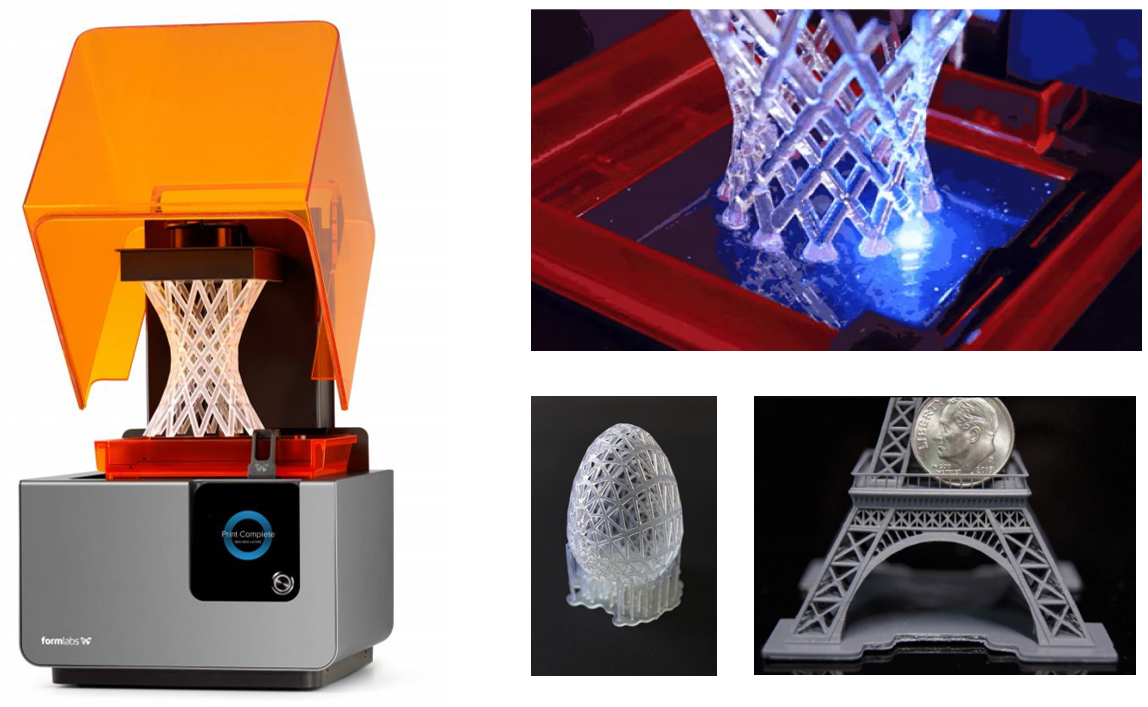
Credit for beautiful photos: Formlabs. If you want to get into the gory details, a resin is composed of at least two different parts: plastic monomers and oligomers, kind of like a glue. They’re sloshing around and not really doing much until you expose them to with a light with a wavelength that excites them, typically UV. Now, a molecule at the end of the monomer and oligometer detach, and the suddenly hot cut ends of the longer chains of these molecules suddenly bond together, in which, we interpret as the substrate hardening, fusing, and ‘curing’.

Stereolithography 3D printing is a form of vat resin printing, where a vat of liquid resin is exposed to a light source to form thin layers of plastic that stack up to form a solid object. The bottom of this resin is a transparent glass window that light can pass through. Between this glass window and a metal build plate is a thin, 25 micron layer of resin that gets cured when exposed. Immediately afterwards, this 25 micron layer is lifted and then lowered back down towards the screen so a new 25 micron layer of liquid can then be blasted with the laser again for the next laser scanning sequence to begin. By precisely guiding light where it need to be across a 2D area, we can harden precise cross sections of a 3D object layer by layer.

Background of Galvos

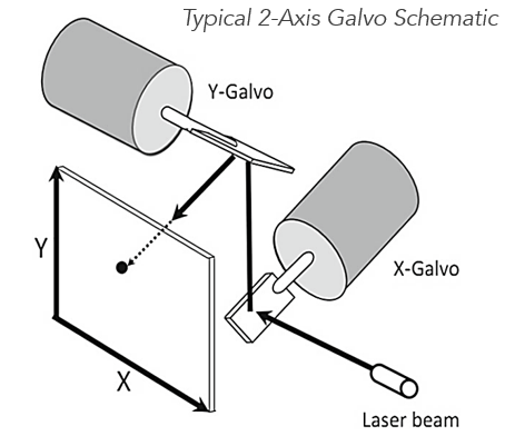
The engine behind this selective light exposure technique is a galvo. "Galvo" is the short name for galvanometer, which is a moving mirror system that steers a beam. A galvo system can be thought as a generalization of crossed fold mirrors, which is a fixed mirror configuration that experiences nontrivial polarization effects when the incident field is converging or diverging. In the case of a galvo, the object field has no such divergence because the laser light is initially collimated. However, the irradiance and polarization state of the beam at each imaged spot varies because each spot location represents a unique path taken through the dynamic system. Alternatively stated, each beam path traverses a distinct sequence of reflections at different AOIs. A typical galvo architecture is shown above, where the fixed laser beam illuminates one fold mirror and then another fold mirror and finally an image plane. Each mirror rotates with the help of a high bandwidth, closed-loop servo motor. As they rotate, they deflect the beam's final position in the image plane.

Potential Effects of Irradiance Non-Uniformity in SLA Printing

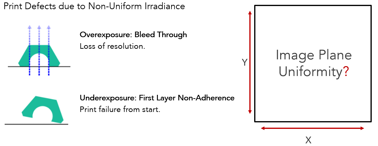
The amount of energy delivered to each curing spot is very important. If the energy delivered to the focal plane is not uniform, then we observe overcuring, where some spots are overexposured to laser light and harden larger areas than predicted by first order design. This ultimately decreases print resolution. Alternatively, spots can be undercured, which means a layer does not fully cure against the build plate, which accrues to print failure. One unfortunate feature about consumer-level SLA printers is that the layer exposure time seems fixed (per layer, at least). To my knowledge, the laser diode current is not modulated and there are no additional compensating optics after the second galvo mirror. This means that any irradiance non-uniformity at the focal plane is not compensated and its impact is directly felt in print quality.

Credit for resin printer defect illustration: AmeraLabs

Polarization has an undeniable effect because SLA galvo-type printers have two mirrors, each of which are weak diattenuators. Diattenuators are elements that have polarization-dependent surface transmission/reflection. Not only that that, they induce retardance because they are metal and their orientations change at every image beam spot. Naturally, the polarization state and output irradiance across the foccal plane will vary across a galvo-scanned image. In lieu of any visualized analyses of these variations in the literature, I wanted to do a polarization ray tracing study in Polaris-M to illustrate the polarization effects of a 2-axis galvanometer scanner. We seek to answer the question: to what extent does polarization play a role in image plane irradiance uniformity of galvo-illuminated scanning systems?

Polarization Ray Trace Modeling

To analyze the polarization effects, I unfortunately could not get the full specs from a 3D printer. However, I was able to get the specs off a Thorlabs galvo, the GVS102. This is a middle of the pack galvo which uses aluminum mirrors and a full scan range of 25 degrees per mirror - likely similar to what we'd see in the Form 1.
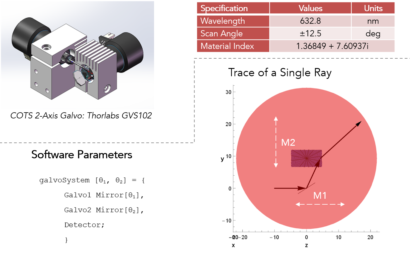As for the software modeling, this system wasn’t traced like a typical image-forming system in Polaris-M. In a typical raytrace, we trace a singular initial distribution of rays at different angles and positions going through a single system. N object rays pass through that single system, but a galvo system instead sends a single aimed ray through N systems to produce each image field point, and holistically, the entire image. My setup approach was to generate each of these N systems and collate the information at the image plane one ray at a time.

In terms of objet placement, I set up my optical system as three surfaces: two mirrors and a fixed image plane, as a function of user-defined tip/tilt angles. Using Mathematica's table function, I generated every system across the mirror rotation range, trace a single ray through it, and collect all of this information for the entire sampling for analysis. To show what a system looks like for a ray specified at a plus 12.5 degree, plus 12.5 degree positioned galvo, you can see the deflection of that ray on the bottom right. M1 steers the beam horizontally across the image plane, and M2 steers the beam vertically.

Image Sanity Check

For a first check, I ran the raytrace for a single input ray across the full angular sweep. Extracting the image plane intercept positions, this is what you get – a distorted rectilinear grid as a function of position coordinates. The distorted pincushion image point mapping distortion occurs because we have a finite distance between the galvo mirrors. If the distance between the crossed fold mirror axes was decreased, we could minimize the distortion. Here the aspect ratio is ~4:3.

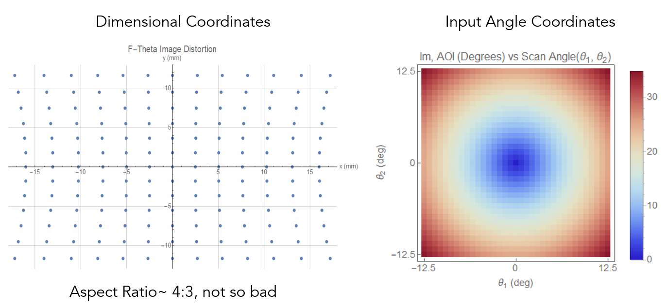
Of interest to us is the AOI (Angle of Incidence) Map, which is shown at the right as a function of galvo scan angle. The maximum AOI at the image plane is 34 degrees and is radially symmetric. For all subsequent maps, I chose to index by scan displacement angle, which ranges from -12.5 to 12.5 degrees, rather than true image spot position. My justification was that keeping the maps as functions of galvo scan angles allows us to discuss them as dependent variables. The image distortion isn’t so bad that we can’t intuitively interpret and dissect the maps anymore.

Effects of M1

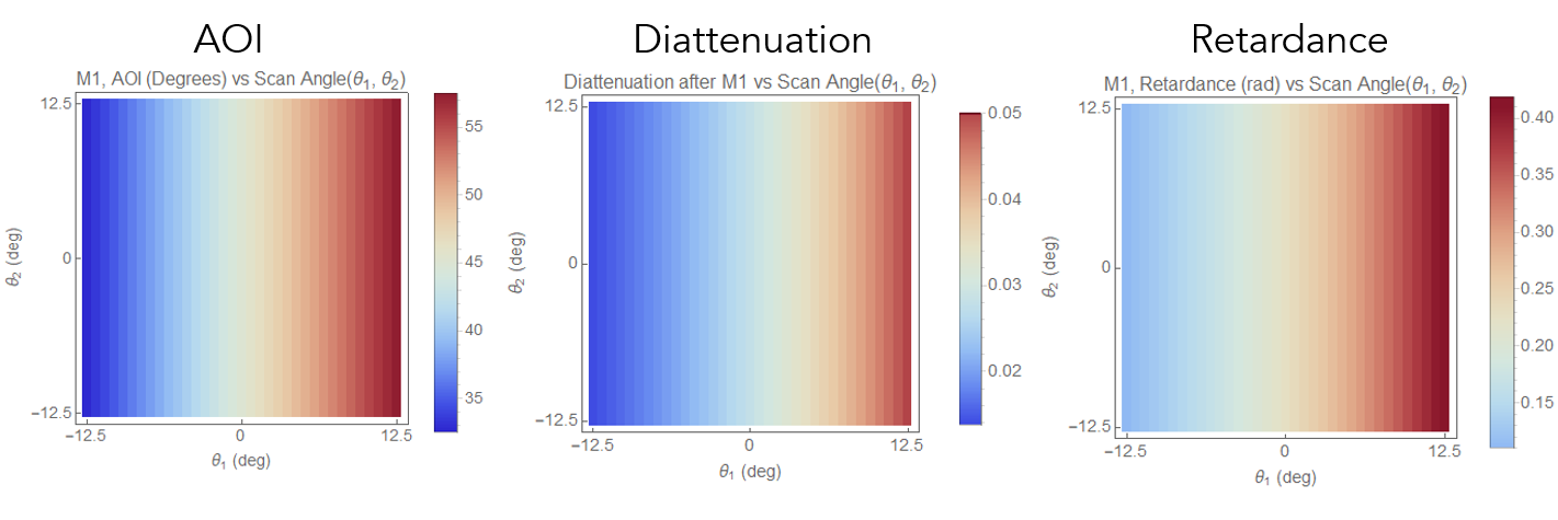
These figures shows the results of the ray trace to the first mirror. (Note again that we are indexing by scan angle, not position, so many of these points can share the same spatial coordinates, but all of them are uniquely indexed by an angle coordinate, Theta 1 and Theta 2.) Given that the scan angle is plus minus 12.5 degrees, it should be no surprise to us that the AOI’s shown by this AOI map vary by exactly that, from exactly 32.5 degrees to 57.5 degrees. Since Fresnel equations are a function of the AOI, it’s intuitive see that the diattenuation and retardance patterns also are spatially similar to the AOI distribution. The diattenuation is up to 5% while the retardance is up to 0.4 radians. These maps indicate that we would observe different amplitude and phase variations based on the polarization state content of incident beam.

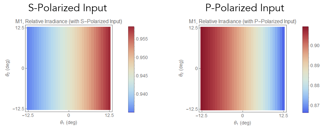
To understand this effect more, we can pass an s-polarized beam and a p-polarized beam through the system and observe their difference after first mirror. Note that s polarized and p polarized are defined with respect to the orientation of the first mirror. The result is that the s-polarized output is higher than the p-polarized output by about 5% across the entire scanning field. This intuitively follows the Fresnel equations, as it should, so far. As AOI increases, s-polarized reflectance increases, and conversely, as AOI increases, p-polarized reflectance decreases.

Effects of M2

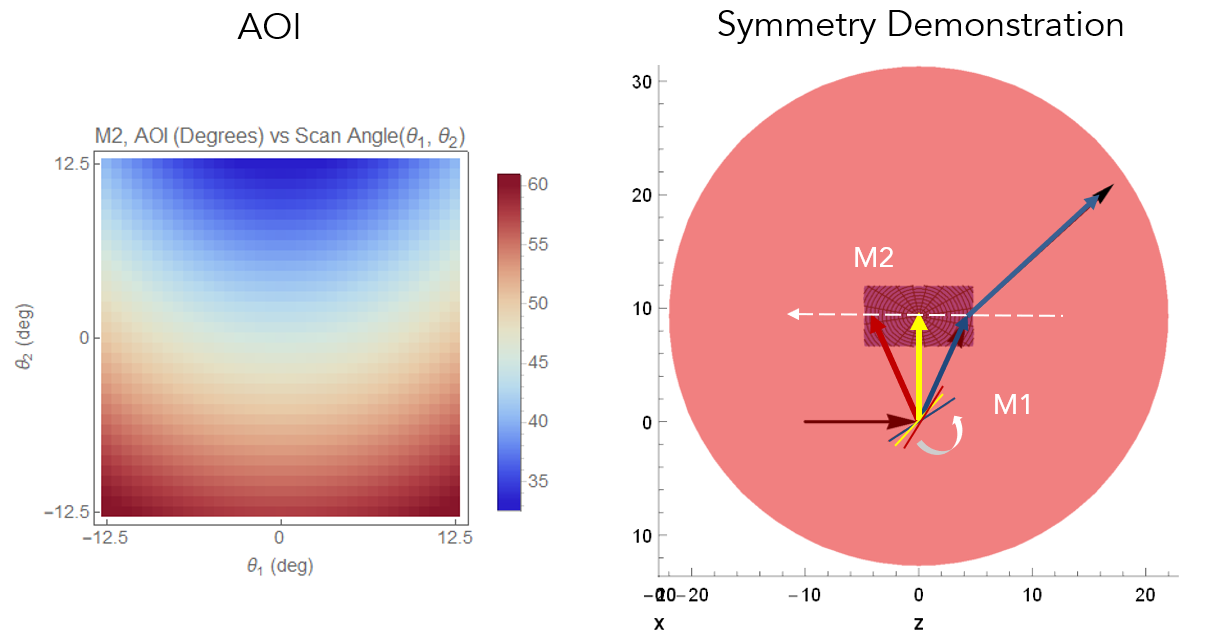
Now once rays hit the second mirror, it becomes significantly less intuitive to interpret what is happening. In the AOI map of M2 on the left, there is symmetry across the irradiance map across the Theta1 axis, but not across the Theta2 axis. To show why that is we can look on the right system printout. If we vary the orientation of M1 in 12.5 degree displacements, we get the blue, yellow, and red vectors respectively each reflecting off their own mirror. As we rotate M1, the beam is only displaced laterally across only this white dashed line. This is all because the incident beam hits M1 at a single point every time because the laser is fixed, and only the deflection angle is changing. We are sweeping a single a line across M2 by varying M1. Now for M2, this observable pattern cannot be similarly generalized because ray intercepts happens across all across this white dashed line. The AOI experienced by each ray not only depends on the orientation of the M2 mirror but also from the angle of the ray from M1 to the M2 intercept. This dependence on M2 intercept position and M2 orientation breaks the symmetry available before.

Where this is confusing talk is getting at is that it is hard to predict how cumulative diattenuation and cumulative retardance will manifest after multiple reflections of a dynamic crossed fold mirror system. There are symmetry breaks, high AOI’s, and the key fact that diattenuation and retardance induced at successive mirrors do not cancel each other out. The results are not intuitively relatable and you NEED to do a polarization raytrace to see all the coupled effects of high AOIs and materials with complex indices. But to anchor down some logic what we we are seeing, we can observe the diattenuation and retardance is 0 at the very center, as it is in a static crossed fold mirror configuration. Also, we see the strongest diattenuation and retardance effects are at the southwest and northeast corners where the galvo was deflected the most.

Global Irradiance Uniformity at Image Plane

Now feeding in two input linearly polarized states: s-polarized and p-polarized, here are the resultant irradiance maps. The most notable feature is a 6% irradiance variation from the southwest corner to northeast corner, which is spatially similar to the previous maps. Across the main diagonal, the there is the least change. Some practical advice from this observation is that if you wanted to 3d print something long you’d want put it across this axis. Across the cross-diagonal we will see the 6% huge gradient so you would not want to print something in that location.

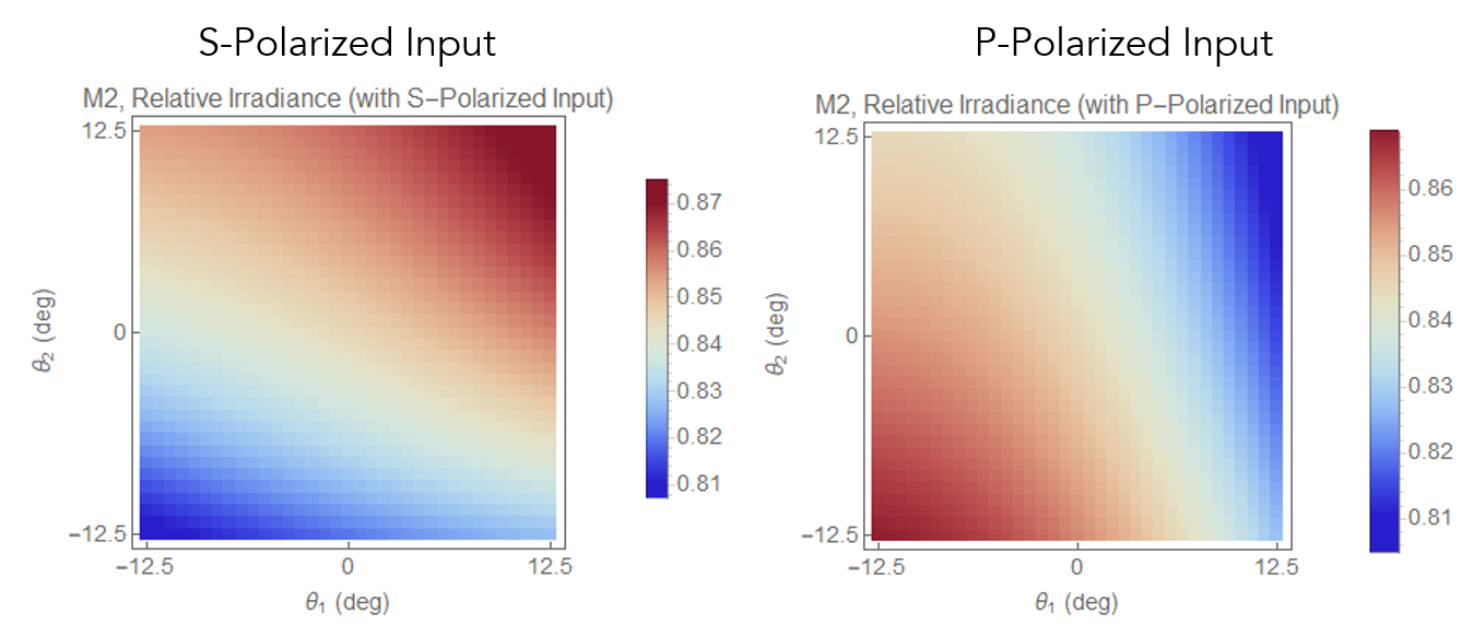
Taking the mean and standard deviation across the maps, observe that the magnitudes of the mean and standard deviation are very much on par. We retain about 84% of the light and have a standard deviation of about 1.5% whether we put in horizontally or vertically polarized light into the system. (To calculate the irradiance, I fed in the s and p-states, got the PRTs (Polarization Ray Traces) of the raytrace indexed by angle, multiplied to get the output polarization states, and then took the dot product of the field and its complex conjugate.)

Regional Irradiance Uniformity at Image Plane

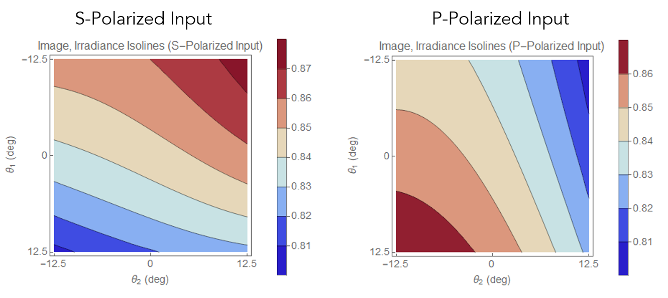
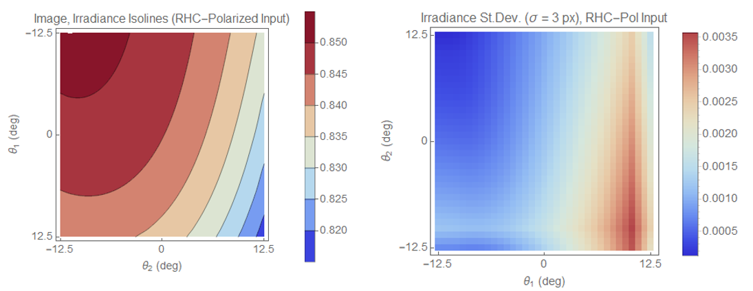
To visualize the irradiance map at the focal plane better, I performed a regional analysis with a contour plot which uses the same color scaling. Zones are separated by relative irradiance differences of 1%, and we can see that the P-Polarized input varies just a little less and has larger zones of uniformity. Like the previous map showed, the only difference is that the gradient of the cross diagonal is reversed between the two input states.

Local Irradiance Uniformity at Image Plane

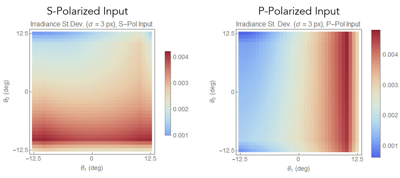
Finally for a local analysis, I applied a standard deviation kernel to look at regional differences. For each pixel convolved, we’ll choose a spatial radius and take the standard deviation of all those values encircled around that center point. I chose a standard deviation of 3 pixels (~2.5 millimeters). Spatially we see tiny variations even across regions centimeters large. Overall, I would say this is pretty good and if you’re 3d printing a small part with 50 millimeters , you could probably put it anywhere on the print bed and quality differences for intra-bed positions would be negligible.

Poincare Sphere Projections

The next thing I wondered was how do all the polarization states (linearly, circular, elliptical, N/A?) changed when you pass an initially linearly-polarized beam into the system. So I also plotted the result of horizontal linearly polarized light into my system and this was my result:

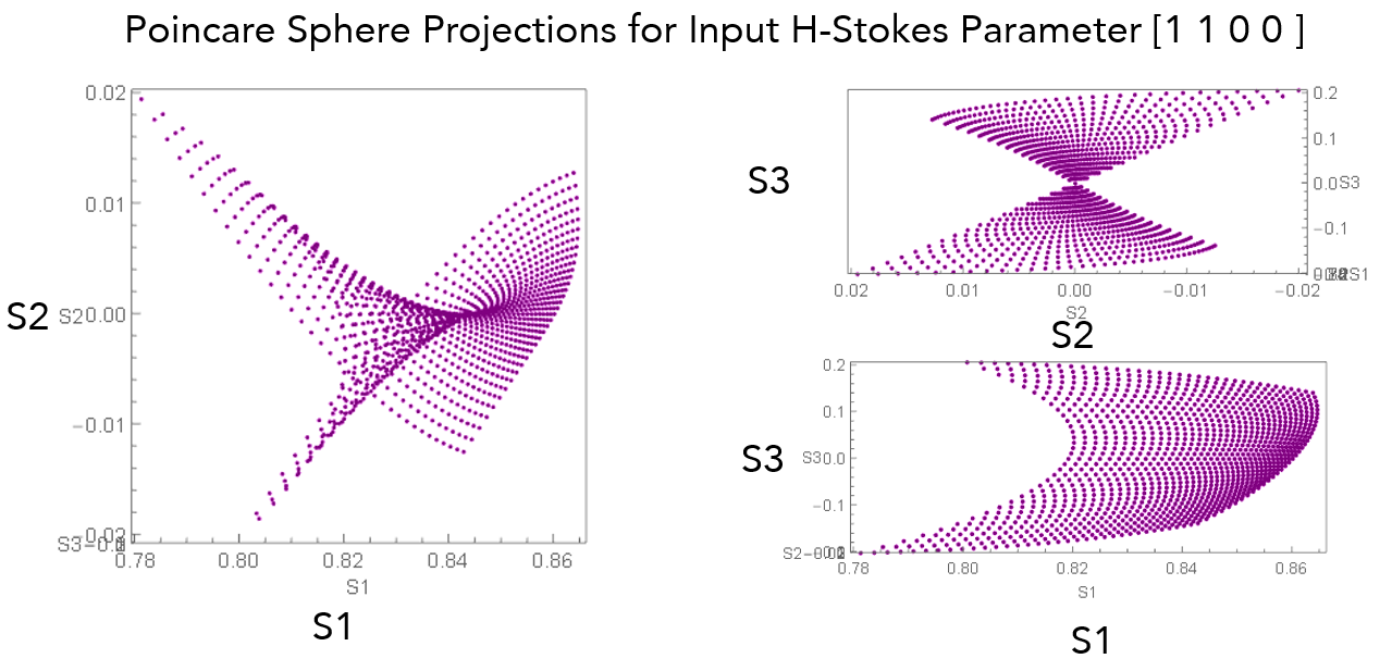
These output polarization states plotted on the Poincare Sphere coordinate system, and then projected onto a plane. I chose to NOT normalize the outputs as I wanted to see the energy losses experienced, so this is NOT a true Poincare sphere representation. Output polarization states seem to make tight folds on themselves and do not at all stay linear. For example, the projection onto the S3 basis reaches a magnitude of 0.2 and has the form of a "Figure 8". This 'stretch' along the S3 axes is characteristic of metal fold mirrors seen in astronomy. A consequence is that if any of the polymers in the vat have polarization sensitivity, curing will be influenced.

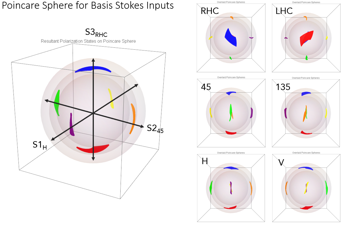
Extending this idea to the full basis set of input polarization states (horizontal linear, vertical linear, 45 linear, 135 linear, right hand circular, left hand circular), I threw these fully polarized states into my system as to observe how their magnitudes and ellipticity would change as a result of propagating to the focal plane. Note that each input spate, which is located at a pole of the Poincare Sphere, produced output states that remained in the vicinity of the pole location that they came from. Circular polarizations were way more uniform and wrapping around a sphere better than any of the linear polarization states. Resultant polarization states of the beam were always ellipticized, with the pronounced "figure 8" warping.

Possible Mitigations and Solutions

Right circularly polarized input, same uncoated aluminum mirror system. Looking at the literature of laser cutting, it is actually no surprise that they introduce a retarder at the beginning of the optical system to improve kerf. A quarter wave retarder oriented at the fast axis converts the polarization of a linearly polarized beam into a circular one. Circular input states end up working better because the projection of a circularly polarized beam rotates rapidly and therefore averages out undesired polarization artifacts as light is incident at each itnerface.The results of circularly polarized input (just mount a quarter waveplate normal to the optical axis of the nominal beam), show improved regions of uniformity across the global irradiance plane and much better local standard deviation. However, the cheapest quarter wave retarders I could get were ~$200, I suspected this would be hard to justify in the system for its performance effects. You'd need to mount this, seal this, deal with any heat effects, and pay for the waveplate itself for marginal improvement.

Same horizontal linear polarized input, silver mirror coating. A semi-final comment is that one can simply choose mirror coatings to improve reflection at the range of applicable AOI's. All the effects I mentioned were only possible as consequences IF no additional dielectric film (MgF2 is interestingly an anti-reflection coating for dielectrics and a high-reflectance coating for aluminum) is added atop the aluminum. You could of course just use a silver coating with super high reflectance to minimize the reflectance variations between the s and p states and get a low variation map because reflection was high no matter what state and angle of incidence characterized a beam.

Realistic Impacts

In general, if an additional coating is NOT put onto an average set of galvo mirrors OR it doesn't use naturally highly reflective coatings such as silver, we will see variation from one corner to another. This is primarily due to the unique series of reflections at each mirror, leading to different AOI's and diattenuation at each interface. I don't know what the Form 1 and Form 2 use, but galvo geometry is relatively invariant so the effects in real system build surfaces will resemble what I have commented on here.

Quite frankly, the polarization effects shown here are small fish compared to the quality performance determinants that SLA printers must get right. It's a hard task and I'm amazed that SLA printers can be sold at $4000 and deliver such good quality. There are so many things that go into print performance, but for profesional (and not just pro-sumer level) printers, polarization must definitely be initially controlled or digitally "flat fielded".

Last Comments

This insidious cross-diagonal variation will also appear in any other galvo systems. For a laser welding system, a long seam weld might show non-uniformity if welded from the southwest to northeast corner of the work area. Laser welding is increasingly used in cookware and surgical instruments because they can hold unusual geometries together with great strength. However, uniform joints are necessarily to establish to proper loading, lest a non-uniform joint introduces an unacceptable failure mode. It is possible that more expensive equipment compensates for this irradiance difference such as external attenuators, but simply, pulse width modulation can help tune the average power until seen fit.

In this polarization ray-trace and analysis, we obtained information about the irradiance variation in an image plane due to the polarizing effects of two crossed metal mirrors. Galvanometer concerns are typically spelled out as laser power variation and spot size variation across an area, but here, polarization effects show that they deserve consideration too.