Henry Quach

Scope of Study

For any surface metrology system that obtains measurement with the aid of an imaging system, distortion must be carefully scrutinized. Both intrinsic lens distortion and perspective distortion embed surface error distributions that skew the interpretation of resultant surface maps. Either displaces acquired information due to the imaging process. Here, we quantify the origins of distortion, its modeling philosophy, and the effects of its digital correction procedure. This study includes simulation for lens-distorted systems such as interferometers and perspective-distorted systems such as monoscopic fringe projection profilometry and deflectometry. Summarily, this study hopes to clarify differences in low-order shape between surface metrology instrument measurements in which surface maps were not rectified for distortion.

Introduction

Imaging, or the process by which a physical scene’s radiance is captured and projected onto a 2D plane, is a fundamental tool in full-field optical surface metrology. Ideal imaging asserts that each object point is uniquely mapped to a single conjugate image point. Mathematically, this transformation preserves the collinearity of points and ratios between lines. Indeed, the remapping of a radiance distribution to an image sensor is useful in interferometry [1], photogrammetry [2], fringe projection profilometry (FPP) [3], and deflectometry [4]. These methods invoke imaging in order to sample measurands like phase, degree of polarization [5], surface slope [6] (which are all later pixel-wise processed to height), or direct height itself at a detector.

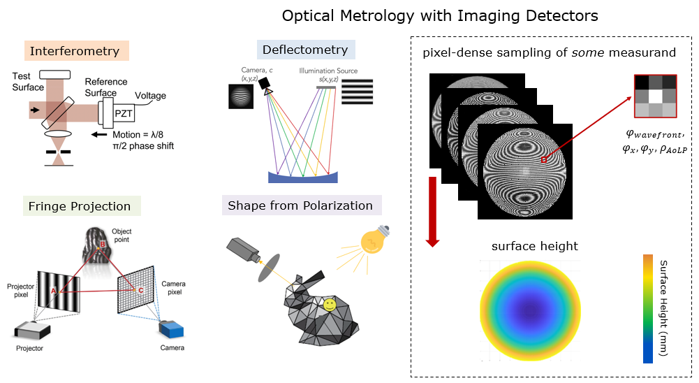
Figure 0a. Different metrology methods that use an imaging camera to sample a test optic.

In practice, imaging a field consisting of physically equally-spaced object points does not create equally-spaced image points. This is due to distortion, or the variation of magnification when objects are imaged through a lens. Variation of magnification with object-to-entrance pupil distance is known as perspective distortion while variation of magnification with object field height is known is lens or “optical” distortion.
So, what is the influence of either type on optical surface measurement? Even a high-quality machine lens with “0.5%” lens distortion observes some difference in surface measurement result if uncompensated. Furthermore, metrology methods that use a single camera to sample information at an object field possess different image magnification distributions based on their orientation and distance relative to an object. We seek to elucidate the influences of common scenarios if uncompensated without metric distortion calibration, or the use of well-located and known physical fiducials to deduce how to transform distorted data into a clear orthographic representation. Instead of this exact vectorial technique, it is common to simply scale an image in the horizontal or vertical direction to transform the image data into its expected shape. To what extent will this common, undistortion technique influence final surface measurement?

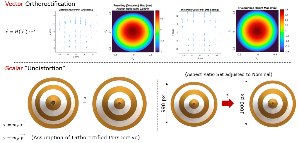
Figure 0b. Vector vs. Scalar rectification processes.

This study explores the influence of distortion and basic undistortion for common optical shapes with an aperture diameter of 25.4 mm, including a f/1 convex spherical optic, f/1 concave paraboloid, tilted plane, tilted object plane with image plane meeting the Scheimpflug condition, and a tilted f/1 spherical optic. Results are presented in representative error maps from original surface heights and trendlines of error coefficients in the Noll Zernike set. [7]

Physics of Lens Distortion

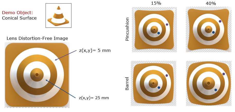
Figure 0c. Example of lens distortion with a traffic cone.

Lens distortion is inherent to the optical imaging system itself; it is the variation of magnification with object field height. When chief rays from points on an object pass through the entrance pupil of an imager, there is variation in the ray slope ubar. Variations in ubar alone do not create magnification variation issues. For example, there is no lens distortion in pinhole cameras because unvignetted rays simply map to the detector with no change in ubar. However, for refractive systems, the non-linearity of Snell’s Law (e.g. the ratio of two sines) inherently gives rise to the nonuniform magnification of chief ray slopes. [8] In symmetric optical systems about the stop, the nonuniform magnification of chief ray slopes is eliminated by cancellation of equal and opposite contributions. Yet this total cancellation of lens distortion is limited to only the 1-to-1 conjugate imaging configuration between the object and detector, limiting general utility in eliminating lens distortion.

The lens distortion inherent to an imager is often given as the following, from the parametric Brown-Conrady model, though many physically-based distortion models have arisen since the popular model’s inception. [9] $$ p_d =[x_d/y_d ]= (1+\alpha_1 r^2+\alpha_2 r^4+ \alpha_5 r^6 ) [x_n/y_n ]+[( 2 k_3 x_n y_n+k_4 (r_n^2+2 x_n^2 ))/(k_3 (r_n^2+2 y_n^2 )+2 k_4 x_n y_n )]$$ The distorted coordinate \([x_d/y_d ]\) is a function of several coefficients (α_n) of an even symmetric power series, plus tangential terms (\(k_n)\). While the origins of this parametric model are not tied to the physical nature of lens distortion, it is frequently sufficient to describe its effects, as fitted by camera calibration.

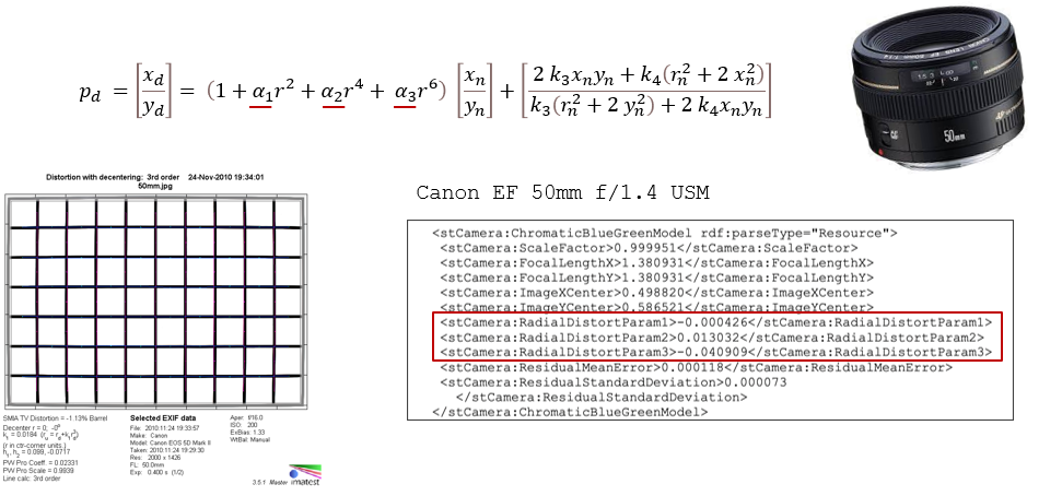
Figure 0d. Lens Distortion of a Real Canon Lens

Physics of Perspective Distortion

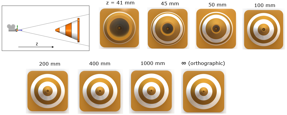
Figure 0e. Example of perspective distortion with a traffic cone

In lieu of pupil aberration, a chief ray begins at an object point and crosses exactly through the axial locations of the entrance pupil (EP), stop, and exit pupil (XP) on the way to its corresponding paraxial image point. From a plane object imaged to a plane image by a paraxial lens, a uniform magnification exists, \(m_{paraxial} =\frac{\bar{u}}{\bar{u'}}=\frac{y'}{y}=\frac{z'}{z}\). Here, both planes are normal to the lens optical axis. The chief ray angles are defined as \(\bar{u} \) and \(\bar{u'}\), field heights defined as \(y\) and \(y’\), and field point axial distances defined as \(z\) and \(z’\) in object and image space, respectively.
However, any object with finite depth \(\delta_z \)viewed by non-telecentric imaging systems produces an image with non-uniform magnification. This is based on how axially distant the object’s constituent points are from the EP. For an ideal imaging lens (with no lens distortion) focused at a datum of a plano-convex test optic, \( y'_0 = m_0 y_0 \) defines the magnification. The object field height \(y_0\) has the paraxial magnification m_0 and image height \(y'_0\). For the same imager and scene geometry, the general magnification relationship \(m_n=y'_n/y_n=z'_n/z_n\) holds for the object field height \(y_n\). Its corresponding image point with height \(y'_n\) is not guaranteed to be in focus, though by definition, it will possess the magnification \(m_n\).

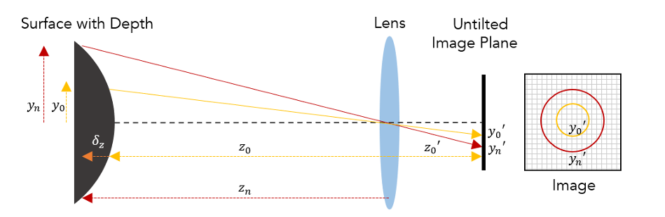
Figure 1. This schematic of an on-axis object being imaged by a paraxial lens demonstrates the angular nature of the chief ray passing through the thin lens, which is coincident with the stop, EP, and XP. Ordinary imaging systems are a boon in that their sloped chief rays create an angular (rather than fixed object area) field of view. This fact allows a lens and detector to observe different magnifications of an object with change in distance from the imaging system.

As shown in Figure 1, for an on-axis object with field-dependent depth \( \delta_z (y_n ) \), its magnification as a function of the reference axial position \(z_0\) is, \(m_{obj, On-Axis} (y_n) =z'_0/(z_0+\delta_z (y_n ) ) \) We may define the relative magnification (d) with respect to \(m_0\) as, $$d_{On-Axis} (y_n )= \frac{m_{obj,On-Axis}}{m_0} =\frac{z'_0}{z_0+\delta_z (y_n)}/\frac{z'_0}{z_0}=\frac{z_0}{z_0+\delta_z (y_n)}$$ This expression quantifies that the variation of magnification is based on the ratio of object depth to object distance. The fixed distance \(z'_0\) but varying distance \(z_n\) intuits that perspective distortion is reduced by larger distances from the camera and also smaller object depths. The ratio of object depth to object-to-EP distance determines the relative influence of perspective distortion.
One exception is in object-space telecentric systems, whose design forces chief rays to be parallel to the optical axis. The non-angular nature of chief rays within object-space telecentric designs therefore eliminates perspective distortion because all chief rays appear to originate from infinite distance. Unfortunately, telecentric lens systems pose different limitations for optical metrology use cases, most notably, that the objective lens must be as large as the object to be imaged.
The perspective-distorted scenario for an off-axis object is more visually apparent and pernicious. Tilts introduce asymmetry into the distribution of the chief ray angles through the EP, altering the image overall footprint (e.g. a circle to ellipse, or rectangle to a trapezoid) as shown in Figure 2. Here, \((y_m,y'_m)\) and \((y_n,y'_n)\) are two pairs of conjugate points that experience different magnifications from the on-axis object point \((y_0,y'_0)\) due to object depth.

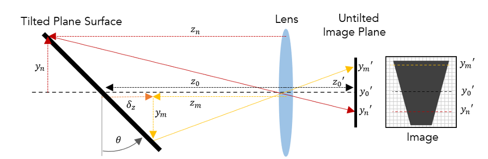
Figure 2. The schematic of an off-axis system tilted by \(theta\) brings forth keystone distortion in the unflipped image of the plane object. If the image is rotated 180°, the ‘foreshortening’ effect is observed, where \(y'_m\) has a greater magnification than \(y_n'\) due to relative proximity.

The relative magnification of image points is calculated again for a tilted object, $$d_{Off-Axis} (y_n )=\frac{m_{obj,off-axis}}{m_0} = \frac{z_0'/(z_0+\delta_z (y_n ) }{z'_0/z_0 }=\frac{z_0}{z_0-y_n tan⁡ \theta} $$ Finally, in a third common imaging scenario, Scheimpflug imaging is described for this perspective effect, illustrated in Figure 3. It resembles the previous case, but unlike for an image plane normal to the optical axis, meeting the Scheimpflug condition achieves focused imaging for the entire tilted plane object onto a tilted detector. Extant keystone is slightly mitigated but uneliminated. $$d_{Sch} (y_n )=\frac{m_{obj,Sch}}{m_0} =\frac{f+z_0}{f+z_0-y_n tan⁡ \theta } $$

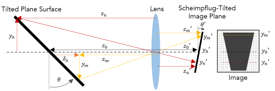
Figure 3. In Scheimpflug imaging, in-focus imaging of an off-axis object is met by tilting the image plane for a specific calculated amount. [10] The specific tilt required for the image plane is \(\theta' = tan^{-1}[z'_0/z_0 \cdot tan(\theta)] \). Because the magnification is negative through a thin lens, the image plane tilt is always in the ‘opposite’ direction as the original object tilt. [8]

Coarse Distortion Rectification

‘Undistortion’ is the name of many processes which rectify the effects of distortion. In the ideal case of precise metric undistortion, we transform a distorted map into an orthorectified map whose grid of pixels represents physical regions of equal areas and true surface information sampled at each pixel. Since points on the distorted maps are assumed to have correct information (just at the wrong position in the imaging plane location), undistortion moves each point to its location by a vectorial mapping. Here, \(\vec{r'}\) is the set of camera image points, \(\vec{H} (\vec{r})\) is the object location-dependent rectification transformation, and \(\vec{r}\) is the set of orthorectified coordinate positions. $$\vec{r}=\vec{H}(\vec{r})\cdot(\vec{r'} ) $$ In practice, the full vectorial mapping procedure usually requires placing physical fiducials at precisely-known locations, \(\vec{r'}\), imaging the fiducials through the camera to \(\vec{r}\), calculating the vectors from \(\vec{r'}\) to \(\vec{r}\), and applying the fitted transformation \(H(\vec{r'})\) across the entire distorted image. [11] Unfortunately, this process is time-consuming and requires expensive equipment (i.e. coordinate measurement machines or laser trackers). We chose to examine the influences of undistortion in its most basic but accessible embodiment: scaling one dimension relative to another (if required) so that the correct aspect ratio is maintained. This transformation resembles the scaling operation, $$\vec{x}=m_x \cdot \vec{x'}$$ $$\vec{y}=m_y \cdot \vec{y'}$$ For example, a circular aperture that is imaged into an elliptical one due to perspective is scaled in one dimension, m_y, to return to its expected circular image footprint. As another example, on-axis imaging of a spherical optic with depth is accepted as a distortion-free map, without any rectification for the variable magnification with depth or radial lens distortion. The scaling rectification process isn’t rigorous but is common, and quantitative studies of this coarse method’s influence on surface measurement were unknown to the authors. We felt that this accessible rectification technique deserved exploration, whether to sway metrology practitioners from its adoption or to justify regimes of its usage.

Methodology for Distortion Simulations

Two programs were built in Matlab to simulate the effects of lens distortion and perspective distortion. One applied radially symmetric lens distortion, and the other applied perspective distortion related to spatially-varying object-to-EP distances and detector plane tilts. In our context, ‘applying distortion’ means to transform a uniform grid of true object point heights at their true spacing to their resultant distorted spacing at the image plane. After the distorted maps are obtained, both programs conducted simple scaling undistortion.
For the lens distortion simulation, only the effects of the radial coefficients \(\alpha_2\) and \(\alpha_4\) were explored since they are prevalent among fitted distortion coefficients from camera calibration. A f/1, f/2, and f/4 optic were modeled, distorted, and then ‘undistorted’ by scaling. The full sequence of steps taken is shown in Figure 4.

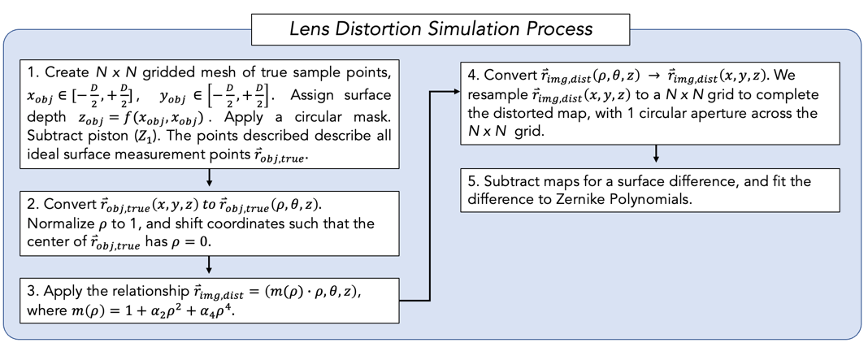
Figure 4. This is the procedure for lens distortion simulation. No ray trace is needed since the lens distortion is based on the radial displacement of points relative to the center of the original object, which is placed on the optical axis of the lens.

As for the perspective distortion simulation, a ray tracer for a generic surface with rays propagating through a pinhole and into a tiltable image plane was built. To account for the magnification inversion, the image was rotated 180° about the optical axis before rectification operations. The full procedure is outlined in Figure 5.

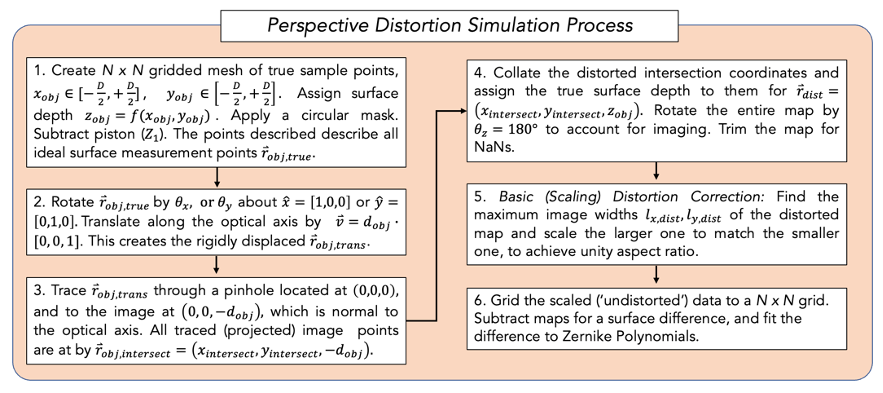
Figure 5. This is the procedure for perspective distortion simulation. A ray trace is necessary to produce the projection effects which create perspective. The image is not necessarily normal to the lens, as it is tilted in the Scheimpflug test case.

A total of 122 lens distortion simulations were run to obtain the lens distortion error trends in the next section, taking ~2.9 seconds per trial. All simulations began with 1001x1001 sampled objects with exact surface heights modeled by their typical conic equations. For ray-traced perspective distortion simulations, 885 trials took ~9 seconds each, obtaining the perspective distortion error trends plotted in the next section. Perspective simulations were run on Matlab 2021a with an AMD Ryzen 7 2700X 8-core processor at 3.70 GHz.

Lens Distortion Simulation Results

To demonstrate the effects of distortion on a common optical surface, we show the result of the lens distortion simulator observing an f/1 convex surface with \(\alpha_2\) radial distortion in Figure 6. For a single-detector metrology technique that samples the correct height of this optic using an imaging system with \(\alpha_2\) =1%, the imaging process will have distorted the sampled points at the image plane. Each sampled point still has the original height information as from the perfect object map, but now in the wrong location within the circular aperture of the image, due to the radial displacement of imaged points. Subtracting the distorted map and original ideal surface, a resultant -4.671 um of Z4 Power and +1.139 um of Z11 Spherical Zernike error would have been interpreted by accepting the unrectified map as-is. Figure 7 shows the trends in Z4 and Z11, when \(\alpha_2\), \(\alpha_4\) are swept from -2 % to 2%. Several microns of Z4 loom at even the 1% lens distortion.

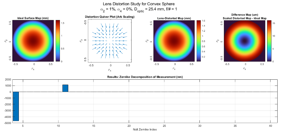
Figure 6. Simulation output plots showing the ideal surface map, quiver plot of distortion vectors (not to scale), lens-distorted map, and the difference map. The ideal and lens-distorted map appear similar, but the difference map shows power and spherical errror.

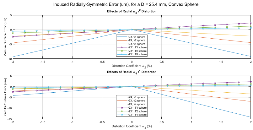
Figure 7. Plotted trends show that the quadratic lens distortion \(r^2\) factor creates significantly more Z4 power error than Z11 spherical error. Conversely quartic lens distortion factor is less influential on surface error when negative, but steeply more influential when positive. Lens distortion of even 0.5% of either create microns of error, which is significant in the context of precision metrology.

Perspective Distortion Simulation Results

To demonstrate the effects of perspective distortion on a f/1 convex surface at 200 mm from the lens, we show the result of the perspective distortion simulator observing it in Figure 8. Object points at the convex surface were propagated through a pinhole stop and chief ray slopes were unaltered as they passed through before intercepting the image plane. The primary result of on-axis perspective distortion is spherical aberration error. Unsurprisingly, the Z11 trends for f/1, f/2, and f/4 convex optics decrease in influence for slower optics and further distances, shown in Figure 9. An f/2 sphere sees less than 1 wave of Z11 when the object is at z = 650 mm. An f/4 convex spherical object scenario saw less than 1 wave of Z11 even at the short object distance z = 100 mm.

Perspective Distortion for a Concave Spherical Object

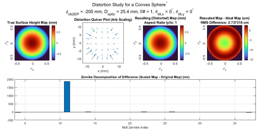
Figure 8. Convex Sphere: Distortion study of imaging an on-axis convex sphere. Actual surface, distortion vector plot, measured surface, and difference map (top). Zernike decomposition of difference map (bottom). Note that the distortion quiver plot is not monotonic in a given radial direction; vectors point both towards and away from the center.

Note that in the trendlines, an object distance of infinity sometimes did not reduce perspective distortion to zero, which should be the case for chief rays parallel to the optical axis. In this case, the finitely sampled circular aperture created fictitious system shape error (which halved every time we doubled sampling) when fitted to Zernike polynomials, so this static error at z_obj=-∞ was subtracted from all data points of a given Zernike trend when present.

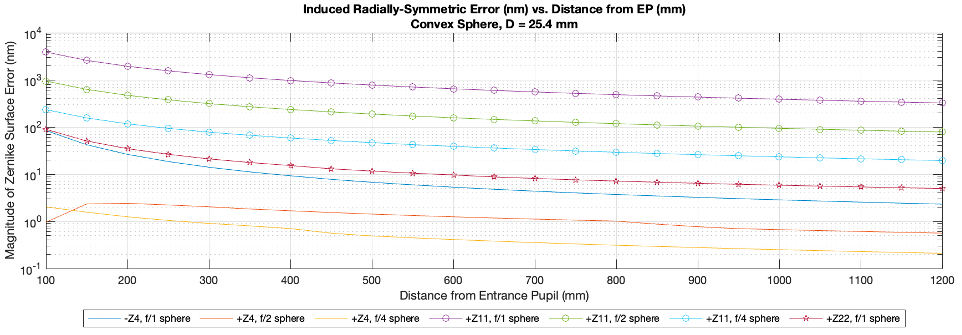
Figure 9. Convex Sphere: Trends of spherical objects for their f/# vs distance for Z4, Z11. f/1, f/2, and f/4. Spherical aberration dominates the induced error, while power error exists in fractions of a wave. Slight amounts of second order spherical aberration (Z22) were present for the f/1 sphere, though tiny for the slower f/# surfaces. For a convex paraboloid, Z11 was also the strong dominant error source, while Z4 error was only 13.56 nm for even the f/1 surface case.

Perspective Distortion for a Concave Paraboloid Object

For a concave paraboloid, almost no Z4 content was induced for all test cases, depicted in Figure 10. Z4 was present at the quantity of only 10.74 nm in the f/1 object case, and 4.60 nm in the f/2 case. This is not due to the conic nature of the object, but the concavity. For example, in a non-included study, a concave f/1 sphere object simulation also showed similar lack of induced Z4 error at all object distances. Only spherical aberration error trends are shown in Figure 11.

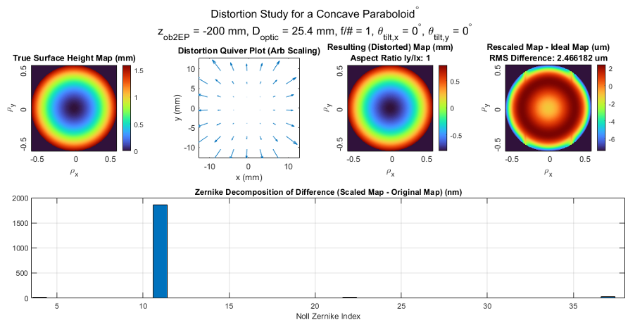
Figure 10. Concave Paraboloid: Trends for objects with their f/# vs distance for Z11. f/1, f/2, and f/4. Actual surface, distortion vector plot, measured surface, and difference map (top). Zernike decomposition of difference map (bottom). The vector displacement points radially outwards. The (Rescaled Map – Ideal) Map has four ‘ears’ which are likely artifacts from grid interpolation and scaling.

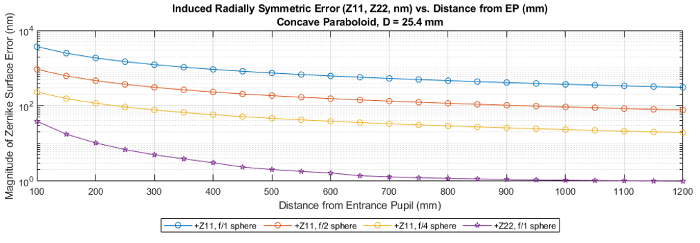
Figure 11. Concave Paraboloid: Trends of f/# vs distance for induced Z11 error. 1st Order spherical aberration is the primary induced error term, while power/defocus error was noticeably absent.

Perspective Distortion for a Tilted Flat Object

The study of a tilted flat with a plane normal to the optical axis of the lens, unsurprisingly, produced low order astigmatism Z6, when the resulting distorted map was undistorted by scaling back into a circle. In Figure 12, note how the the resulting distorted map becomes vertically ellipticized after the projection through the pinhole and onto the image plane. The distortion quiver plot demonstrates just how uneven the magnifications between the upper and lower portions of the imaged points are. Scaling distortion rectification is insufficient because the magnification change between adjacent image points in the vertical direction is non-uniform. Thus, a linear scaling operation cannot undo the non-linear mapping induced by the perpsective transformation. Astigmatism trends for various object tilt angles is plotted in Figure 13.

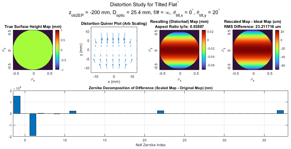
Figure 12. Tilted Plane Object with a Circular Aperture: trends for flats with their tilt angles vs object distance for Z6. Actual surface, distortion vector plot, measured surface, and difference map (top). Zernike decomposition of difference map (bottom). Z6 astigmatism was the dominant error, with 19.098 microns induced due to the scaling distortion rectification.

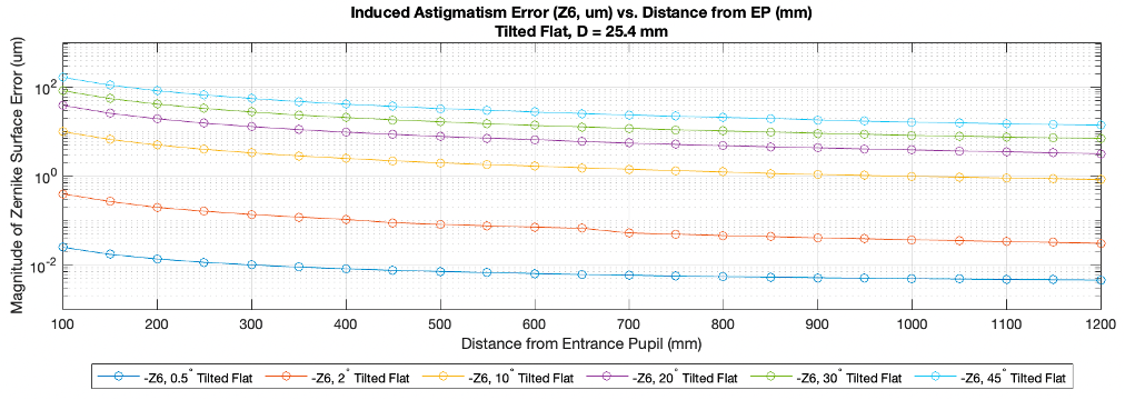
Figure 13. Tilted Plane: Trends in object tilt angle vs. distance to EP for Z6. Only the case of a 2° tilted flat experiences 1 wave or less of Z6 at distances 200 mm or further from the EP.

Perspective Distortion for a Tilted Flat with Image Plane at the Scheimpflug Condition

Imaged at the Scheimpflug condition, the distortion quiver plot (Figure 14) is strikingly different from that in Figure 12. Radial symmetry of the distortion vectors was re-established by tilting the image plane. Note that keystone still exists, as the vectors around the vector plot are not entirely equal in magnitude. Unfortunately, the effects of a tilted plane to achieve proper image focus does not reduce Z6 astigmatism error. Though this imaging configuration introduced image tilt \(\theta'_y = -2.316^\circ\), Z6 remained at ~ 20 um. Figure 15 demonstrates similar trends in astigmatism reduction with object distance to Figure 13.

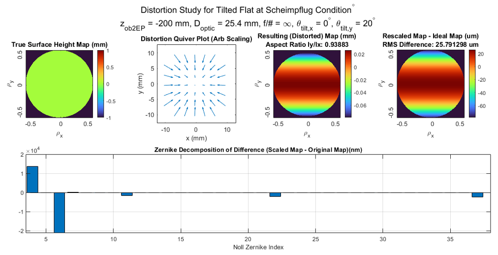
Figure 14. Tilted object plane with the detector tilted in the opposite direction to meet the Scheimpflug condition: Distortion study of imaging on-axis convex sphere. Actual surface, distortion vector plot, measured surface, and difference map (top). Zernike decomposition of difference map (bottom).

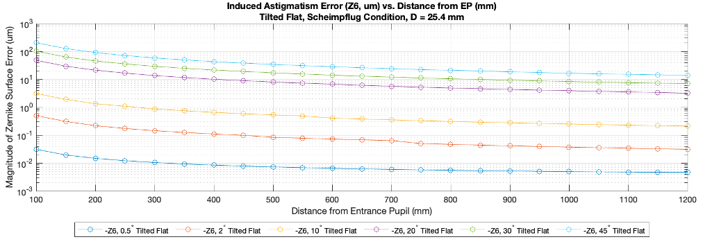
Figure 15. Tilted Plane at Scheimpflug: Trends in object tilt angle vs. distance to EP for Z6. It remains that only the case of a <2° tilted flat experiences 1 wave or less of Z6 at distances 200 mm or further from the EP.

Perspective Distortion for a Tilted Convex Sphere Object

The final persective scenario images a tilted object with depth. In Figure 16, the influences are quite varied: coma is introduced for the first time and as a significant error contributor. The distortion quiver map is both asymmetric and not monotonic. The centroid of the resulting distorted map is no longer at the center of the square map. Figure 17 shows the astigmatism and coma trendlines.

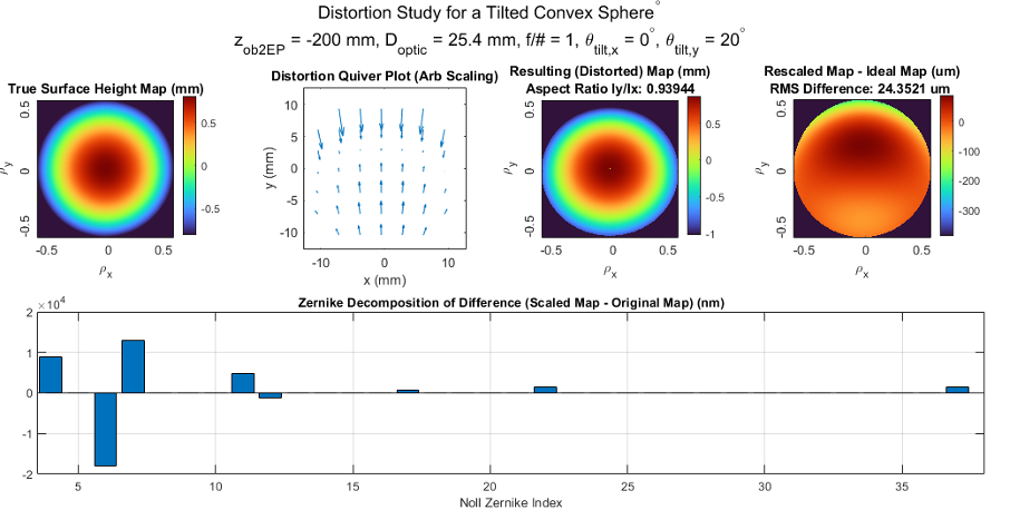
Figure 16. Tilted Convex Sphere: Distortion study of imaging on-axis convex sphere. Actual surface, distortion vector plot, measured surface, and difference map (top). Zernike decomposition of difference map (bottom). The Zernike decomposition includes power, astigmatism, and coma. The rescaling undistortion operation translates the shifted centroid of the distorted map as the elliptical image footprint returns to a circular perimeter.

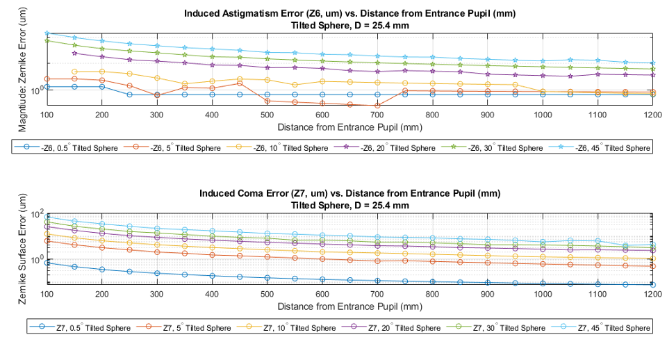
Figure 17. Tilted Plane: Trends in object tilt angle vs. object distance to EP for Z6 Astigmatism and Z7 Coma. In the trendlines for the -Z6, 5° Tilted Sphere and -Z6, 10° Tilted Sphere cases, trends appear to fluctuate in magnitude, perhaps due to fitting or interpolation issues. Error remains well above 1 micron of coma and astigmatism except for the 0.5° cases. The impact of perspective distortion for a tilted object with sag is not as easily interpretable as the previous four cases.

Discussion

For at 25.4 mm diameter optic, a convex f/1 spherical optic, concave f/1 paraboloid, tilted plane, tilted plane with image plane meeting the Scheimpflug condition, and a tilted /f1 spherical optic were studied for induced aberrations (Z4 Power, Z6 Astigmatism, Z7 Coma, and Z11 Spherical) against tilt angle, f/#, and distance from object to entrance pupil. Some interesting takeaways from the data were:
Lens Distortion: on a convex surface, quadratic lens distortion \(\alpha_2 r^2) \) creates significant Z4 power error and some Z11 spherical error (2-3X less than Z4). Quartic lens distortion \(\alpha_4 r^4) \) induces Z4 surface error when \(\alpha_4 \)is positive rather than negative. At least 2 microns of Z4 error is anticipated for an imaging lens with \(\alpha_2) \)= 0.5%.
On-Axis Perspective Distortion: for both concave and convex spherical optics, Z11 spherical error was dominant induced error. When imaging a f/2 sphere through a distortion-free lens, there is only less than 500 nm of Z11 error induced when the object is 650 mm away. Z4 error was nearly non-existent for concave surface simulations due to the compensating effects of geometry.
Off-Axis Perspective Distortion: if a flat is imaged 10° or more off-axis from the lens optical axis, then a minimum of 10 microns of Z6 astigmatism will be present. Here, scaling distortion rectification is insufficient because the magnification change between adjacent image points in the vertical direction is non-uniform. Thus, a linear scaling operation cannot undo the non-linear mapping induced by the perpsective transformation.
Off-Axis Perspective Distortion at the Scheimpflug Condition: tilting the image plane to achieve conjugate imaging did not effectively reduce keystone distortion. The magnitudes of induced Z6 were commensurate with cases with untilted image planes. However, the distortion quiver maps now show striking radial symmetry, while the vectors from the non-Scheimpflug case highly varied in magnitude along the direction of the plane tilt.
Off-Axis Perspective Distortion for a Convex Lens: Tens to one hundred microns of Z6 astigmatism and Z7 coma were the result of imaging a tilted object with depth. The influence of the tilt was complex and demonstrates the need for sophisticated orthorectification techniques.

Conclusions

In this study, the modeling of intrinsic lens distortion and physics of perspective distortion were described. Then, a lens distortion and ray-tracing perspective distortion simulator were built in Matlab to model the influences of unrectified distortion on surface metrology instruments that use a camera to sample measurands at a surface under test. The simulations applied a distortion to ideal surface height data at an object, and used a simple scaling rectification method to undistort the distorted image data back into its expected shape.
Overall, the study motivates true metric distortion calibration rather than scaling. True metric distortion places physically well-known fiducials across the sampled object field, so that the mapping between true physical space and distorted image space may be obtained, fitted, and applied. Simple scaling rectification hits a hard limit of microns of error if invoked, and must be carefully weighed against the costs of implementing metric distortion calibration. Some next directions in this study of perspective distortion towards sampling height measurands include the fitting of data to various vector orthonormal polynomial sets versus physical fiducial placement error, determining the error induced by physical radius-to-pixel scaling, and exploring vision ray calibration for distortion rectification. [12]

References

[1] Smythe, R., “Practical aspects of modern interferometry for optical manufacturing quality control: Part 2,” Adv. Opt. Technol. 1(3), 203–212 (2012).
[2] Surrel, Y., “Some metrological issues in optical full-field techniques,” Interferom. XI Tech. Anal. 4777(June 2002), 220 (2002).
[3] Feng, S., Zuo, C., Zhang, L., Tao, T., Hu, Y., Yin, W., Qian, J. and Chen, Q., “Calibration of fringe projection profilometry: A comparative review,” Opt. Lasers Eng. 143(August 2020), 106622 (2021).
[4] Huang, L., Idir, M., Zuo, C. and Asundi, A., “Review of phase measuring deflectometry,” Opt. Lasers Eng. 107(August), 247–257 (2018).
[5] Wolff, L. B., “Polarization vision: A new sensory approach to image understanding,” Image Vis. Comput. 15(2), 81–93 (1997).
[6] Huang, R., Su, P., Su, T., Zhao, Y., Zhao, W. and Burge, J. H., “Study of camera lens effects for a deflectometry surface measurement system: SCOTS,” JTu5A.7 (2014).
[7] Noll, R. J., “Zernike Polynomials and Atmospheric Turbulence.,” J Opt Soc Am 66(3), 207–211 (1976).
[8] Smith, W., [Modern Optical Engineering, 4th ed.], McGraw-Hill, New York, NY (2008).
[9] Wang, J., Shi, F., Zhang, J. and Liu, Y., “A new calibration model of camera lens distortion,” Pattern Recognit. 41(2), 607–615 (2008).
[10] Schwiegerling, J., “Scheimpflug Condition Derivation,” 2016, https://wp.optics.arizona.edu/visualopticslab/wp-content/uploads/sites/52/2016/08/Scheimpflug.pdf.
[11] Novak, M., Zhao, C. and Burge, J. H., “Distortion mapping correction in aspheric null testing,” Interferom. XIV Tech. Anal. 7063(2008), 706313 (2008).
[12] Bothe, T., Li, W., Schulte, M., Von Kopylow, C., Bergmann, R. B. and Jüptner, W. P. O., “Vision ray calibration for the quantitative geometric description of general imaging and projection optics in metrology,” Appl. Opt. 49(30), 5851–5860 (2010).