Henry Quach

Background

Structured illumination is a common approach to optical surface measurement. If a light source of known radiance illuminates a surface under test, the light scattered toward a detector often contains information about that surface, albeit encoded. In fact, extracting surface slope or depth via a sequence of structured illuminations is precisely possible with a well-designed illumination configuration and decoding scheme. Measurands such as parallax movement, raw intensity (scaled irradiance at the detector focal plane), or polarization ellipticity/degree of polarization, encode this surface geometry information. Examples of these methods broadly include photogrammetry, interferometry, and deflectometry.

One variation of structured illumination is phase-shifting, which encodes phase across the source. Phase is the absolute cyclic position of a phenomena over its repeating motif. In our context, a light source inherits and exhibits some sinusoidal distribution that varies from a minimum to maximum and back to its minimum, repeating this motif across the source's full spatial extent. In the example of a sinusoidal fringe being displayed across a planar illumination screen in a single direction, a single period spans \(2\pi\) radians of phase in that direction. The brightness at each pixel corresponds to a unique phase value. However, if the single-period motif pattern required four periods to cover the source's spatial extent, then \(8\pi\) radians would be the full range of absolute phase values encoded across source. Clearly, a single intensity measurements of the screen, or of a specular test surface reflecting the screen, is insufficient to obtain absolute phase values.

In this scenario, a temporal sequence of acquisitions where the phase of the sinusoidal pattern is shifted can be used to obtain a wrapped phase. With a fixed phase shift step size, say four steps of \( \pi/2\), the intensity captured at each pixel of the detector can be entered as arguments of an equation that solves for unwrapped phase, usually the arctangent of a sum of intensities over a a different sum of acquired intensities at different phase steps. Encoding phase is popular strategy for structured illumination today, at least for deflectometry and profilometry, because planar sources with spatially-varying and precisely modulated radiance are commercially available and phase unwrapping techniques relatively mature. Regardless of how the phase modulation scheme is mechanically expressed by the light source, i.e. a LCD screen, a projector or piezoelectric actuator, the mathematics of phase-shifting algorithms remains identical. What differes is the real nature of source non-linearity, detector non-linearity, and SNR.

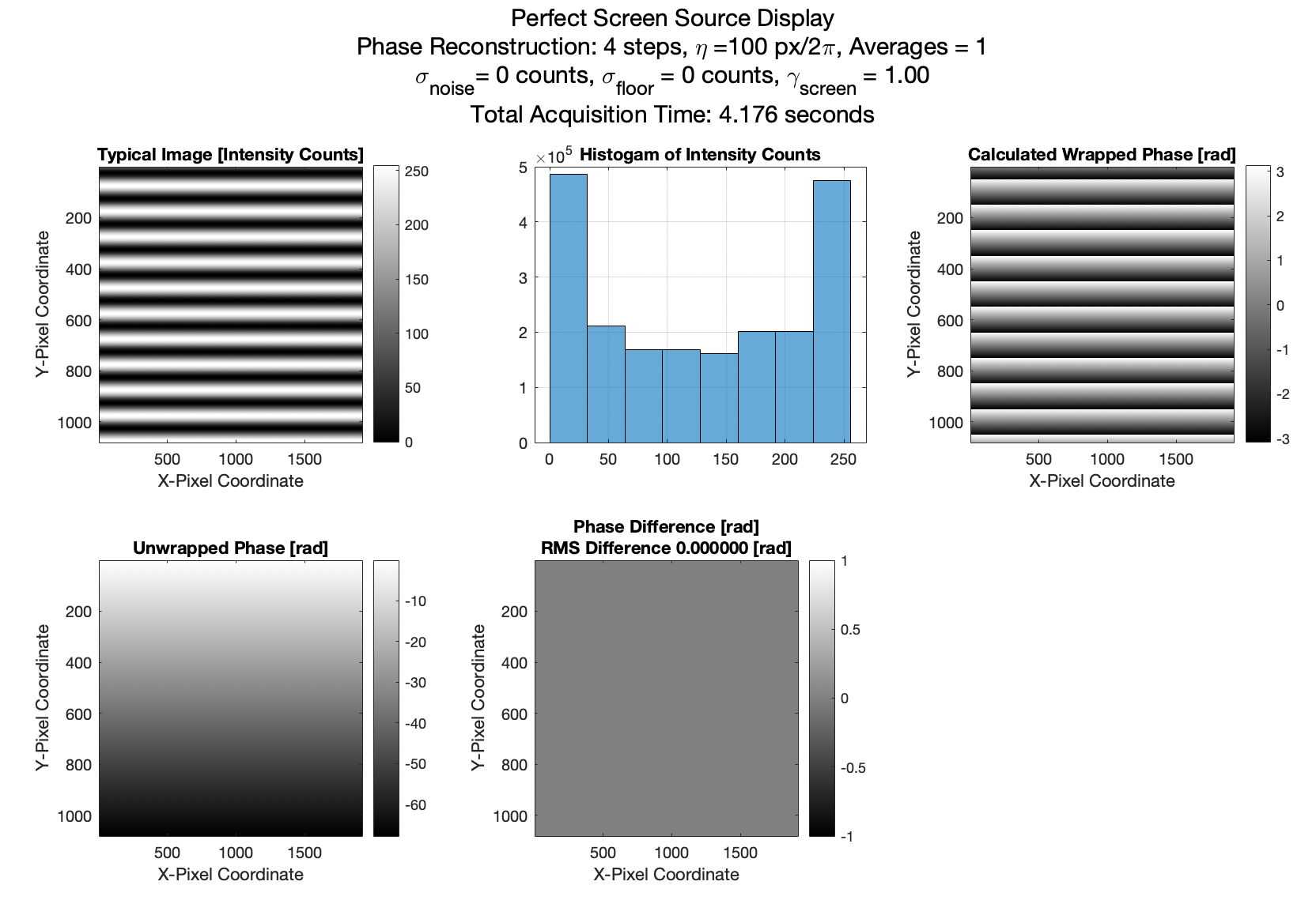
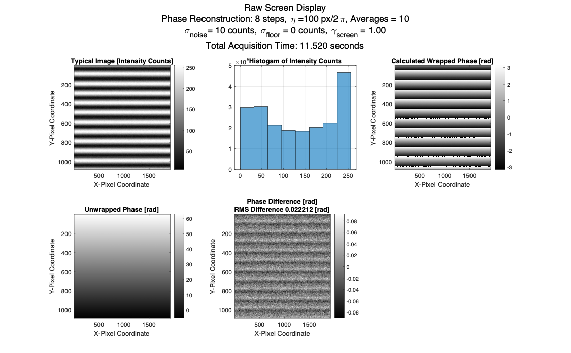
Figure 1. Wrapped phase, Unwrapped phase, and typical sinusoidal motif. Phase difference shows the error in phase wrapping reconstruction with no noise, the ideal case.

Truly, the design of phase-shifting algorithms to decode sequences of phase images fascinatingly complex and stunningly elegant. There has been much research invested into phase-shifting algorithms to decode unwrapped phase, in light of the realities of measurement. This short post seeks to express some of the design elements behind what simply appears to be an arctangent calculation.

Mathematical Preliminaries

For a planar source with a sinusoidal phase pattern in one direction, each pixel posseses the following desired brightness: $$I_n(x,y)=a(x,y)+b(x,y)cos[\phi(x,y)+\delta_{shift}]+\epsilon_{noise}(x,y,t)$$

If we digitally commanded the screen pixel to display ‘128’ brightness counts, we would like the radiance of that pixel to be twice that of when set at ‘64’ brightness counts. The linear scaling of this behavior is desirable, and ideal for the calculation of phase. In PMD, a camera* will capture a sequence of images of the UUT while the illumination screen displays a sequence of phase-shifted sinusoidal patterns. From the set of images, it can calculate phase at each pixel with the N-step algorithm. $$\phi_{wrapped}(i,j)=-arctan\left(\frac{\sum_{k=1}^{N}{I_k(i,j)sin(\frac{2\pi k}{N})}}{\sum_{k=1}^{N}{I_k(i,j)cos(\frac{2\pi k}{N})}}\right)$$ Here, \(N\) is the number of phase steps, so at every pixel captured by the detector, we calculate a wrapped phase in X and Y, \(\phi_{x,\ wrapped},\phi_{y,\ wrapped} \). This calculation shows some basic information about the importance of acquiring well-behaved \(I_i(x,y)\).

1.       We want \(b(x,y)\) to be large, or have high contrast, to decrease measurement uncertainty. \(a(x,y)\) should be designed to sit at the center of the range of b.
2.       Smaller values of \(\delta_{shift}\) means more samples, which, by sampling theory, improves calculation certainty. However, this increases the total acquisition.
3.       We want \(\varepsilon_{noise}(x,y,t)\) to be as low as possible.

In absence of screen effects, this is what we would optimize for. To resist noise, we usually increase the number of steps or the number of averages for each intensity frame image.Some other basic formalities for realistic errors and compensation, include gamma and averaging, $$I_{out,screen}(x,y)=A{I_{input,\ screen}}^\gamma(x,y)+I_{noise\ floor}$$ For \(N\) phase shifts and \(k\) averages, summing intensity images, $$I_{frame}(i,j)=\frac{1}{K}\sum_{k=1}^{K}{I_n(i,j)}$$ 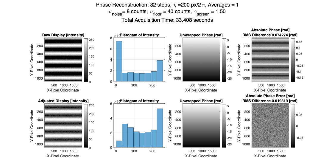One example of phase shifting with typical noise and finite contrast is shown in the figure below. The elements of this ‘perfect’ simulation include: A sinusoidal fringe pattern simulator for the screen, for some pixel pitch \(\eta\ \text{[pixels/full fringe]}\). This fringe is made of pixels with true intensity at 256 brightness levels, [0,255]. We can change the maximum contrast of the pattern to emulate the effect of defocused blur. Available contrast usually reduces to ~0.85 in an acquisition, because the camera focused at the mirror, not the display screen. We can shift the fringe by an arbitrary phase. The phase appears to move upwards/downwards along the y-axis. A phase calculation with the N-step algorithm, which you are familiar with. A phase unwrapping algorithm. This uses Asundi’s reliability-guided unwrapping method.

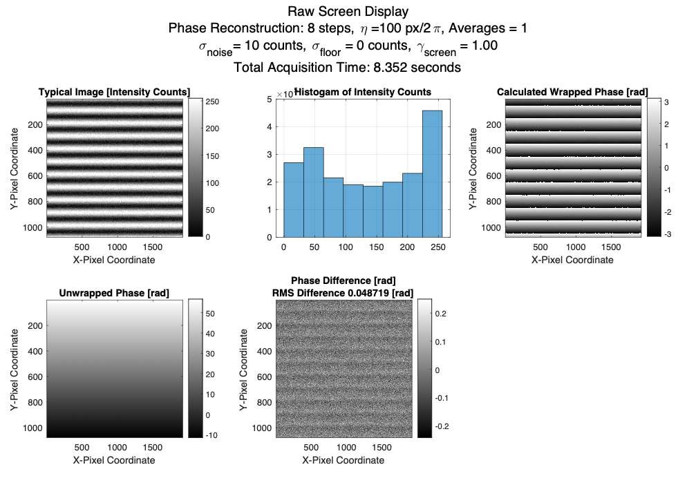
Increasing the number of averages, we can observe immediate effects. The RMS error goes down with phase steps, about halved.

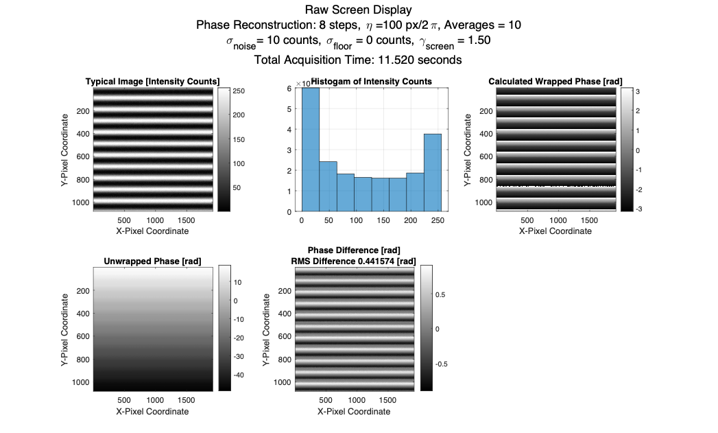
With gamma, we can see the influence on overall phase calculation error. It is horrific, but to be fair screens usually have \( \gamma \approx 2.2\)>. I used \( \gamma = 1.5 \) since that is what I have historically measured on iPad Pros and decent LCD computer monitors. The phase difference grows so large at \( \gamma = 2.2 \) in my simulation that the phase unwrapping breaks.

First, it seems we can mitigate gamma by increasing the number of phase steps. However, if we sweep the number of phase steps, the RMS error reductions are asymptotic. Gamma compensation takes the form of finding and calibration a few coefficients for the non-linear brightness output versus input. We apply the calibrated relationship between screen input and output. $$I_{digital\ input}={{(I}_{output}-I_{noise\ floor})}^{1/\gamma}$$ The next figure shows the difference of assuming linear screen behavior and gamma behavior which is then calibrated out.

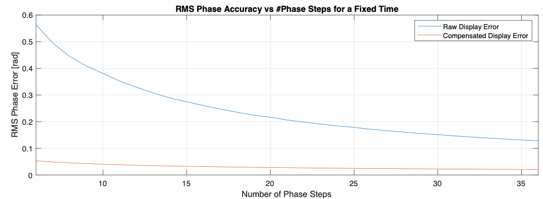
A straightforward implementation of a gamma compensation results in the comparison and times savings.

Some Fourier Theory

This section details some of the beautiful fourier theory behind the scenes of a phase calculation algorithm. I was specifically compelled to write this after reading Yves Surrel's Design of algorithms for phase meassurements by the use of phase shifting, in Applied Optics. Between Hariharan's, Creath's, and de Groote's famous algorithms, what is the commonality and differences? Surely an averaging of phase steps as the argument of the traditional N-Buckets technique cannot be the only way to design and differentiate between algorithms for phase misstep and noise immunity. Actually the differences have roots in characteristic polynomials.

Surrel begins by describig the recorded intensity as a Fourier series. $$I(\phi) = \sum^{\infty}_{m=-\infty} \alpha_m \text{exp}(im\phi)$$ Introducing a phase shift, we can separate the unknown phase to solve for and the known phase step as independent functions. $$I(\phi + \delta) = \sum^{\infty}_{m=-\infty} [ \alpha_m \text{exp}(im\phi)\text{exp}(im\delta)] = \sum^{\infty}_{m=-\infty}\beta _m(\phi) \text{exp}(im\delta)$$ The phase shifting algorithm naturally takes the form, with \(a\) and \(b\) referring to coefficients depending on the phase shifting algorithm. $$ \phi = tan^{-1}\Bigg[ \frac{ \sum^{M-1}_{k = 0}b_k I(\phi+k\delta)}{ \sum^{M-1}_{k = 0}a_k I(\phi+k\delta)} \Bigg] $$ Surrel advises that we can also interpet the phase shifting algorithm, critically as, $$ S(\phi) = \sum^{\infty}_{m=-\infty} \bigg[ \alpha_m \text{exp}(im\phi) \sum^{M-1}_{k = 0} c_k \text{exp}(im\phi)^k \bigg] = \sum^{\infty}_{m=-\infty}\alpha_m \text{exp}(im\phi)P[exp(im\delta)] $$ 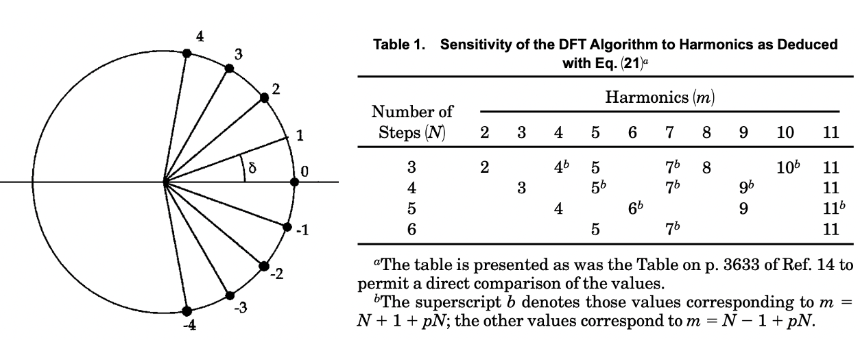What is critical here is Surrel has identified \(P(x)\) as the characteristic polynomial. He clarifies that all properties of any given phase-shifting algorith mcan be deduced from the examiantion of the roots of P(x). The number of coefficients is exactly equal to the number of intensity values involved in the algorithm. $$ P(x) = \sum^{M-1}_{k=0} c_k x^k$$ This inherently shows that insensitivity to certain harmonics is based on the location of the roots, expressed in the complex plane. For example, the equation for \(S(\phi)\) can be rewritten as a Fourier Series as, $$ S(\phi) = \sum^{\infty}_{m=-\infty} \gamma_m \text{exp}(im\phi)$$ $$ \gamma_m = \alpha_m P[\text{exp}(im\delta)]$$ Surrel notes that the necessary condition for insensitivity to a harmonic is \(P[\text{exp}(im\delta)] = 0\), where \( m = -j, ..., -1, 0, 1, ..., j\). To be discussed more in detail are the following figure from Surrel's paper relating roots, overlapping roots, and sensitivities to harmonics: