Henry Quach
Optical EngineerRendering Studies in SolidWorks
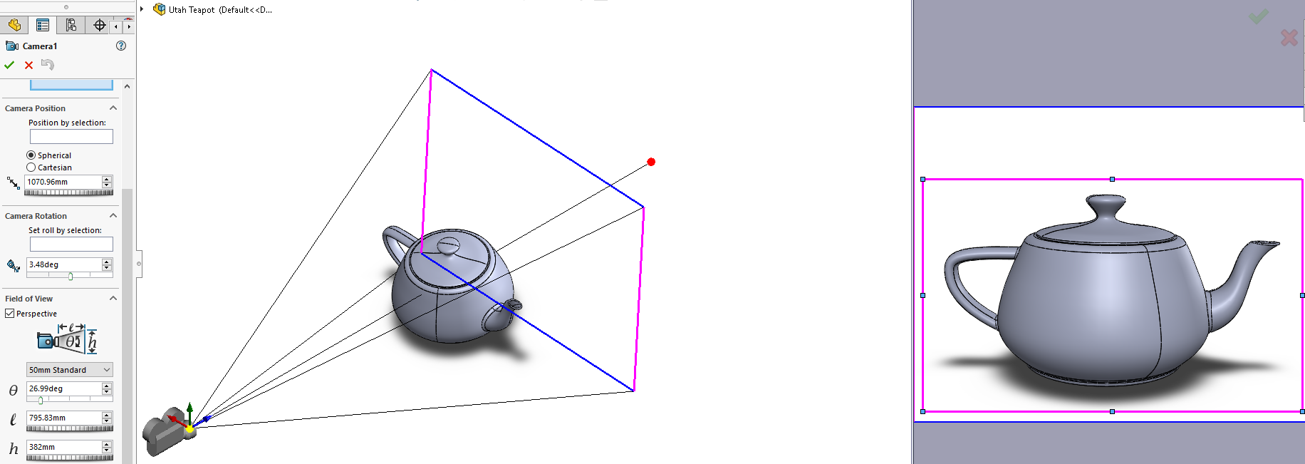
I learned to raytrace in SolidWorks long before I learned to do so in actual optical raytracing software. For fun, I put together several SolidWorks renderings of the famous Utah Teapot to demonstrate the effects of different lighting conditions and BSDFs. The Utah Teapot NURBS surface was downloaded from GrabCad and converted to a sldprt file. I used the MODO rendering environment by Foundry (licensed as Photoview 360 by Dassault) to set up the raytrace and obtain pretty images.
Illumination Model Setup
Illumination modeling requires an illumination source, scene or objects with assigned surface characteristics, and a camera. Here, the camera was preset to a standard 50 mm focal length lens using the pinhole camera model, with an option for depth of field. A 1280 x 1024 detector was set to capture the image. Illumination was not directional, but rather, from a uniform 3D background with a set radiance of 1 W/sr*mm^2. As for setting the shadow, I put a diffusely-reflecting bottom plane 3 mm below the teapot.
Rendering Quality Settings
One of the options in the rendering studio is between 'good', 'better', 'best', and 'maximum' quality. The difference is pretty intense - 'better' often takes 6x longer than 'good'. This is due to sampling curves for better antialiasing (more samples per unit surface area means curves are less jagged), sampling rays to get sufficient SNR at the least irradiated camera pixel, and allowing for more refractions/reflections (up to 32) for each launched ray.
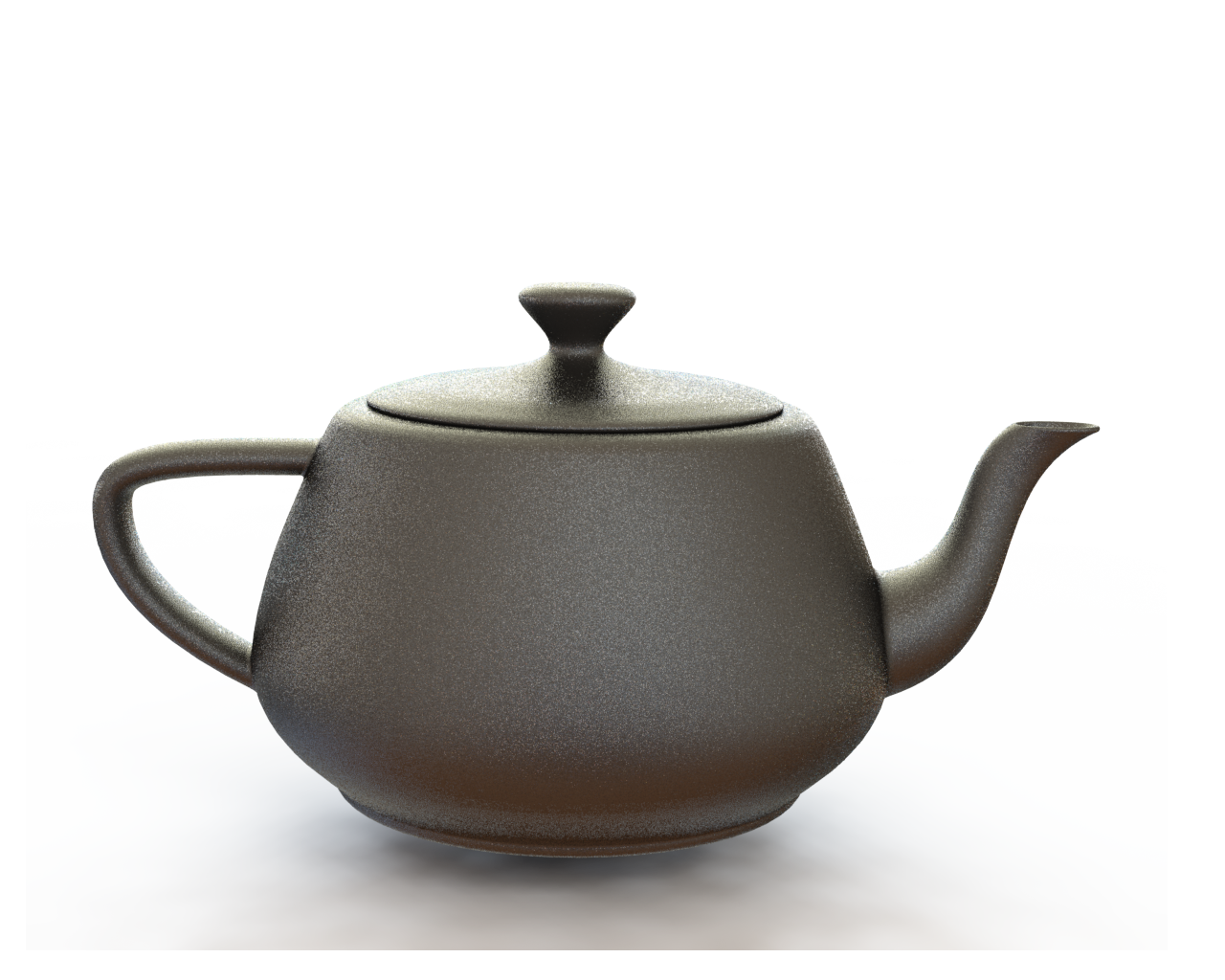
Fun Surface BSDF Comparisons
Please refresh this page if the fun little slider has not shown up!
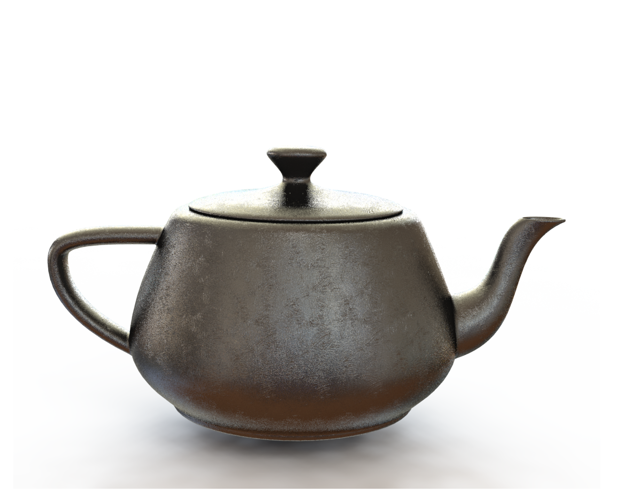
Left Side
Right Side
What's the difference between all of these?
Scatter is the interaction of light with small scale structures, such as edges and gratings - isotropic, anisotropic, and random. It is one of the origins of stray light and explains why rough surfaces reflect light into directions outside the specular angle of incidence. It explains exactly why objects made of the same material but by different processes appear differently.
First described by Fred Nicodemus, the bidirectional scatter distribution function (BSDF) is a function of four variables. The BSDF describes the scattered radiance per unit incident irradiance, as a function of input and output angles in spherical coordinates. Accordingly, the units are in inverse steradians.
$$BSDF(\theta_i,\phi_i,\theta_s,\phi_s) = \frac{dL_s(\theta_s,\phi_s)}{dE_i(\theta_i,\phi_i)}$$
For high precision optical surfaces, it is desirable to minimize scatter so that a light ray remains deterministic and lossless in the direction of desired propagation. In the ideal scenario, a specular interaction has a plot of intensity [W/sr] vs incidence angle [rad] that resembles the dirac delta function. A basic physical example of this is a collimated beam of light impinging on a perfect flat mirror surface and reflecting without increasing the divergence by any infinitesimal arcsteradian, thus conserving Étendue.
In reality, all interactions between light and an interface are a mix of diffuse and specular behavior. The scatter is generally centered about the specular angle, falling off towards larger angles. The figure below, on the left, visualizes the scatter intensity output relationship for several exiting specular reflection angles.
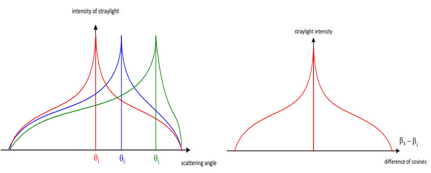
Figure: University of Jena, Advanced Zemax Modeling - Harvey-Shack Theory
Jim Harvey noticed that radiance \(L(r,\theta,\phi)\) could be obtained by dividing the intensity by the cosine of the scatter angle and results in symmetry, as per the right figure. Taking this representation further, if the radiance is plotted against the sine of the scatter angle minus the sine of the specular angle \( |\sin{\theta}-\sin{\theta_0}|=|\vec{\beta}-\vec{\beta_0}| \), physical scattering data appears plausibly linear shift-invariant (LSIV). The observation implies the existence of a surface transfer function (STF), which is applicable even at high scattering angles.
Harvey's model is strictly an empirical formulation and provides a method for compact representation of optical surface if 1. surface roughness is isotropic and 2. the scale of surface roughness is small compared to the wavelength of incident light. Richard Pfisterer of Photon Engineering gives a back-of-the-envelope specification as 1% of the probing wavelength. Putting in real numbers, he provides the figure that 2 nm RMS, which is common among commercially polished surfaces, easily satisfies this condition.
ABg Modeling for Isotropic Surfaces
As a result of the high applicability of Harvey's model to commercial optical surfaces, an empirical ABg model is widely used. The etymology of the ABg model originates from the fitting variables used to characterize a set of BSDF measurements, obtained with a goniometer. In a typcal representation of the ABg model, a loglog plot visualizes the quantity \(log (BSDF)\) as a function of \(log( |\vec{\beta}-\vec{\beta_0}|)\).
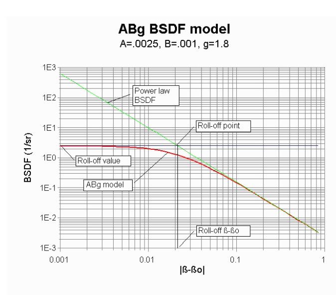
Figure from: Lambda Research Corporation - An Introduction to Scattering and the Surface Property in TracePro
The ABg Model Fitting Form
$$ BSDF(|\vec{\beta}-\vec{\beta_0}|) = \frac{A}{B+|\vec{\beta}-\vec{\beta_0}|^g}$$
\(A\) is the total integrated scatter, \(TIS\), or the 'specular peak' numerator variable. \(P_s\) is the scattered power, while \(P_0\) is power in the specular direction.
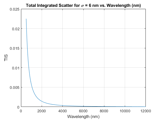
$$ TIS = \int_{0}^{2\pi}\int_{0}^{\pi/2} BSDF(\theta_i,\phi_i,\theta_s,\phi_s)\cos(\theta)\sin(\theta) d\theta d\phi$$ $$ = \frac{P_s}{P_0+P_s} \cong \frac{P_s}{P_0} $$ $$ \cong \left( \frac{4 \pi \sigma \cos{\theta_i}}{\lambda} \right)^2$$
In the limit of \(A = 0\), no scattering occurs, and is obtained directly by integrating a goniometer measurement's of power into a hemisphere.
\(B^{1/g}\) gives the angle where the BSDF transitions from a costant value to a power law falloff. \(B\) is the 'specular peak' denominator variable, which is 2 \(\pi\) minus the correlation length. Since near-specular measurements are difficult, the transition angle is actually guessed as a 0.0001 to 0.01 radians from \(\theta_0\). The ratio \(A/B\) defines the maximum value of the BSDF (leftmost on the plot, where scatter is most specular). BRO's handbook on ASAP mentions that \(A\) and \(B\) are both constrained to be greater than or equal to 0.
\(g\) is a both quantitative and directional fitting parameter and is not restricted to a sign.
* To provide intuition towards physical values, \(g=0\) for a perfect Lambertian (and diffuse!) surface. This implies that the quantity \( |\vec{\beta}-\vec{\beta_0}|^g\) is constant, which makes sense because the obtained radiance is constant, as expected for a Lambertian surface.
* Increasing the value to \(g > 0\), one can see that the BSDF falls off with inceased scatter angle because the quantity \( |\vec{\beta}-\vec{\beta_0}|^g\) in the denominator grows larger with \(g\). Pfisterer notes that \( 1.5 < g < 3.5\) for many polished optical surfaces, where \(g = 1.5\) is a common value.
Examples of BSDF
The purpose of this section is to show the BSDF of various materials to provide additional intuition about scattering. I used Zemax's BSDF library to show how the BSDF varies, and in no way, do I own any of this data - it is represented here to simply show how BSDF is fitted to physical goniometer measurements with the ABg model.
Common BSDF Distributions
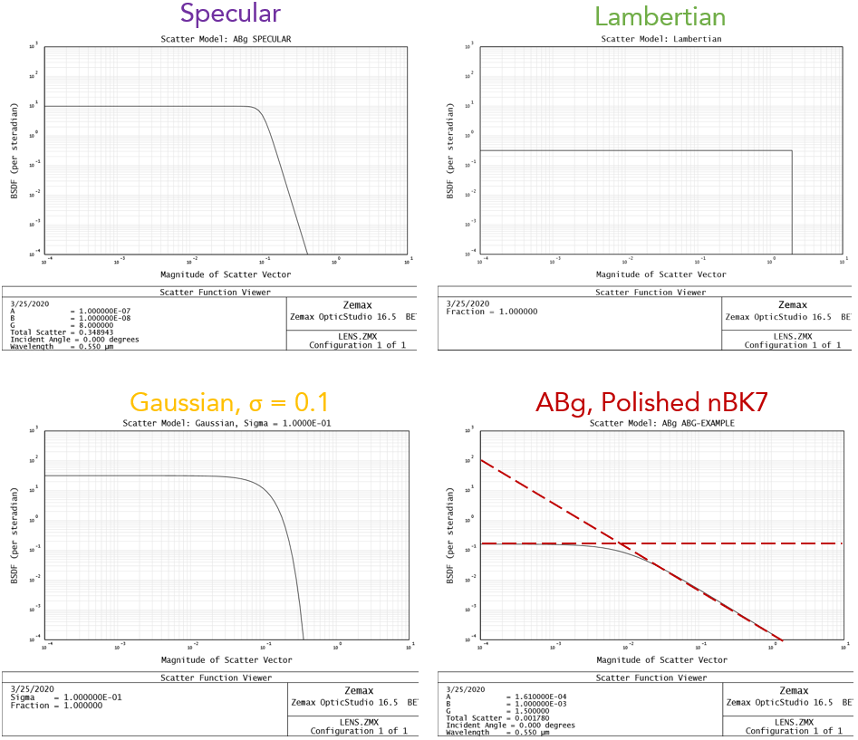
Note the relative characteristics in the above figure: the highly specular distribution has a tall plateau and drops off at a scatter angle of much less than 1 radian. The Lambertian distirbution is fo course constant thru the maximum scatter angle, \( \theta = \pi/2 [rad] \). The specular Gaussian model has the same \( (A/B) \) value as the specular, but its dropoff is slightly more gradual than the specular. Finally, the ABg model for polished NBK7 remains highly specular, but drops off at the knee.
ABg BSDF Distributions
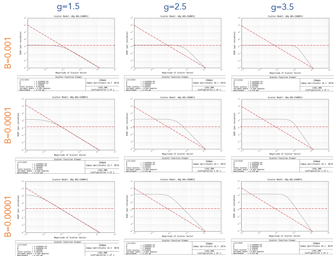
Finally, in the ABg model, I swept the variables \(B\) and \( g \). Dashed red lines are same among all loglog plots, and show how increasing \(g\) increases the slope of the logarithmic dropoff and decreasing \(B\) increases the ratio \( A/B \), increasing the overall height of the specular response.
Wavelength Scaling
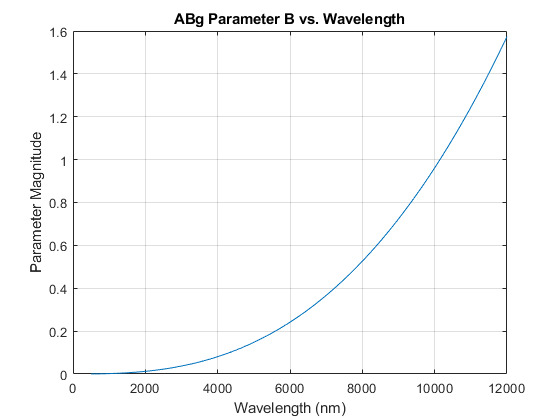
Stover cautions that wavelength scaling is tricky due to bandwidth considerations during measurement. Using Rayleigh-Rice theory of a smooth, clean, and reflective surface (not necessarily Gaussian and conductive), Stover puts an arbitrary line of wavelength been 100 times larger than surface roughness for sufficient smoothness. In the Zemax manual, A and B coefficients are scaled by two equations. Lambda Research Corporation has a really nice justification for why this can be used - it is related to the Power Spectral Density of the surface rougheness.
$$A' = A\big(\frac{\lambda}{\lambda_{ref}}\big)^{g-4}$$
$$B' = B\big(\frac{\lambda}{\lambda_{ref}}\big)^{g}$$
When A and B are plotted, you can see that \(A\) and the total integrated scatter is inversely proportional to wavelength, while \(B\) increases dramatically with it
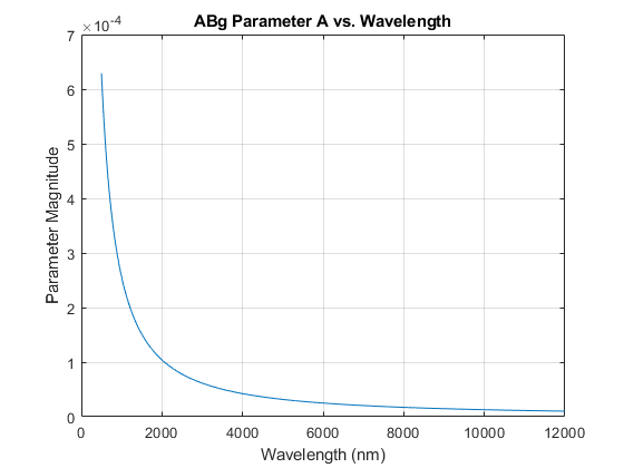
The TIS going down with larger wavelength makes sense because the total power reflected is equal to the specular component plus the TIS. As wavelength increases, the amount of power diffusely reflected goes to the specular component instead. Locally rough patches to a smaller wavelength appear like a smooth planar surfaces element to a wavelength much larger.
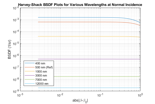
To show the change in BSDF with larger wavelength, I plotted the BSDF of Alanod 5011GP from the TracePro catalog, when obtained from a scatterometer at the normal orientation. This was measured in the visible with the light source being a halogen lamp. The knee of the curves with lower wavelengths manifests themselves near the right end of the plot, while the curves belonging to longer wavelengths remains nearly flat. The significance is that for these longer wavelengths, the curve is magnitudes smaller - the TIS is almost nil and all the reflected energy lives in the specular direction.
Modeling Anisotropic Scatter
Life is so hard. Machined, turned, and milled surfaces have micro or nano-structure features that diffract light with a wavelength similar or smaller than the surface feature scale. ASAP provides several options to account for this, which extends Harvey's model to multiple directions, based onto goniometer measurements from different directions. I could not find more papers about this implementation.