Henry Quach

Introduction and Scope of Study

This analysis project is principally intended to analyze a single canonical lens form, the Tessar. The Tessar is an anastigmat that routinely achieves f/2.5 - f/3.5 speeds while correcting for all seven third-order aberrations. The Cooke Triplet accomplishes the same feat with fewer degrees of freedom, but its performance is more limited. With four elements, the Tessar is perhaps the most manufactured photographic lens form in the world and has a reasonably complex design for potentially engaging discussion. I will be examining design tradeoffs of Tessar against the Cooke Triplet and Double Gauss forms, in terms of aberration correction, relative illumination, distortion, modeled in Zemax.

I'm also interesting in designing and optimizing two very different Tessars: one for machine vision analysis of 3D printed parts during the build process and the second for use as a prime lens during a high-speed Safari chase. Why not??? The optomechanical design of the lens mounting will take the form of a stepped barrel assembly, modeled in SolidWorks. Finally, stray light performance (glare, ghosts) of both designs will be performed in LightTools.

Figure 1. The following starting prescription (f/4.5, f = 100 mm) is provided as a design template from Zemax OpticStudio and visualized using the GLOW module from ELEOptics.

Surface	Type	Radius (mm)	Thickness (mm)	Glass	Diameter (mm)
Object	Standard	\(\infty\)	7.413	-	\(\infty\)
1	Standard	35.034	3.567	N-LAK9	18
2	Standard	-296.111	2.286	-	18
3	Standard	-63.028	2.290	F2	12
4	Standard	31.297	2.289	-	12
5	Standard	\(\infty\)	1.999	-	9.3
6	Standard	-86.620	2.286	K10	16
7	Standard	45.344	9.941	N-LAK9	16
8	Standard	-43.567	86.917	-	16
Image	Standard	\(\infty\)	-	-	38.05

Design Cues and the Modern Design Process

Some key design cues are common to the basics of lens design. For example, a thin lens model that satisfies the desired design power and spacings solve for focal length, Petval Sum, lateral color, and axial color:

$$\Phi_{design} = \frac{1}{y_a}\sum^{k}_{i=1} y_i\phi_i$$

$$ \frac{1}{\rho_{Petzval}} = \sum^{k}_{i=1}\frac{\phi_i}{n_i}$$

$$ \partial_{\lambda}W_{111} = \sum^{k}_{i=1}\frac{\phi_i}{\nu_i}y_i\bar{y}$$

$$ \partial_{\lambda}W_{020} = \frac{1}{2}\sum^{k}_{i=1}\frac{\phi_i}{\nu_i}y_i^2$$

The Tessar and Cooke Triplet bear resemblance because these air-spaced anastigmats have a negative meniscus in the middle. The visually-apparent modification from the Cooke Triplet lay in the rear cemented doublet, which begins its unoptimized surface as a flat at the air-to-glass interface and has equal biconvex (opposite signed) curvatures for the remaining two surfaces. The recommendation by Gregory Hallock Smith finds the doublet's air-to-glass surface will not significantly change after optimization for spot size and OPD, so it may very well be worth to keep the frontal flat surface a non-variable during the entire design process.

We'll start by looking at the patents USP 1,588,072 (F/4.5 Tessar, 28 deg HFOV), USP 2,165,328 (F/3.0 30.1 deg HFOV), USP 2,854,889 (F/2.8 25.2 deg HFOV), and USP 2,995,980 (F/2.7, 16.2 deg HFOV). My understanding of the modern lens design process is that the starting point is the review of patent and template literature, rather than raw third-order theory. A starting design considers the required f/number, wavelength, number of elements, and types of surface (re: manufacturability, cost: not every project can justify an asphere). Starting designs are first optimized for the right focal length, f/number, and system dimension requirements. Lens curvatures and thicknesses also need to be optimized before moving onto glass selection, which also consider cost, availability, and Abbe number. A merit function is constructed next, which must be designed carefully, lest optimization variables descend and ascend forever in endless local extrema.

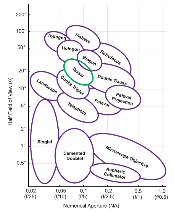
Figure 2. From page 27 of Julie Bentley and Craig Olson's Field Guide to Lens Design, this map of refractive design forms conveniently visualizes design canons that achieve certain HFOVs and f#/NA. For visible spectrum imaging optics, the Tessar occupies a design space with a decent field of view and NA with just four elements. Because most of these canons do not have ambitions for diffraction-limited performance at the production level, it would be interesting to read about the most critical tradeoffs made for performance or against cost.

Sampling, Resolution, and Imaging Quality Goals

An interesting discussion before figuring out the lens designs for either case is first deciding on a sensor. This is sort of arbitrary, but part of the fun. For the safari camera, we'll choose the 35 mm full-frame sensor, which is 36 x 24 mm, and in this case will capture 8 megapixels of information. This works out to 3,264 x 2,448 pixels, with 1.1 micron pixels. For the industrial metrology camera, we'll go with the 1/1.8" format, at 3,088 x 2076 pixels, with 2.4 micron pixels.

Richard Youngworth's paper, 'To zoom or not to zoom: do we have enough pixels?' explores the dual limitation of sensor and optical system resolution. That is, the limitations of incoherent diffraction and maximum signal frequency that can be reconstructed from discrete samples (as foretold by signal processing fundamentals). The mapping from an object point to a image point-spread function directly influences the available contrast at the focal plane. This can be represented with an MTF curve, which visualizes the contrast ragainst object spatial frequency. Richard Juergens has a fantastic presentation on MTF and image quality if you're interested in that. The Nyquist-Whittaker-Shannon Sampling Theorem posits that the maximum reconstructable signal will \(f=\frac{1}{2p}\), be where \(p\) is the pixel pitch.

$$ f_{inc. cutoff} = \frac{1}{\lambda \cdot F/\#}$$

$$ f_{Nyquist} = \frac{1}{2 \cdot p}$$

Indeed, if we have a sensor selected, we want to make the most of its resolution if we are still allowed to play with the design. Youngworth borrows the Q metric from the milieu of remote sensing. In this case, we want sensor sampling to be a little bit more limiting than optical blur, or \( 1.0 \leq Q \leq 2.0 \). The scenario is generous because we are not generating a zoom lens design. Another thing to consider is that we want color pictures for the safari Tessar and monochromatic images for the industrial vision camera. The safari Tessar will require a Bayer filter and pixels will have an effective pitch of 2.2 um rather than 1.1 um.

$$ Q=\frac{2_\cdot f_{Nyquist}}{f_{inc. cutoff}}=\frac{\lambda \cdot F/\#}{p}$$

Radiometric Considerations

We will also consider the radiometry of each imaging scenario. Recall the on-axis image plane irradiance for a uniform, Lambertian object, \(E'\), possessing Lambertian radiant exitance \( M(\vec{r}) = \pi L\). This scenario describes the propagation of energy through an aplanatic lens at finite imaging conjugates. At infinite conjugates, \( m = 0\), of course, and the working f-number becomes the more acceptable regular f-number.

$$ E_{on-axis} = \frac{\pi L}{4(1-m)^2 (f/\#)^2} = \pi L (NA)^2.$$

For an off-axis, Lamberitan source, we also consider natural vignetting:

$$ E_{off-axis} = \frac{\pi L \cdot \text{cos}^4 \theta}{4(1-m)^2 (f/\#)^2} = \pi L (NA)^2 \text{cos}^4 \theta$$

The origins of this equation is actually Etendue. The radiative transfer of power from a small object area to a small image area preserves the \( A \Omega\) product.