Henry Quach

Introduction

Across fields that require precise measurement, it is desirable for an optical system to produce images that accurately portray a captured object or scene. If a set of images can preserve a scene radiance’s and scale between object features, it is possible to extract reliable information or even reconstruct 3D models from them. However, a common obstacle to achieving these ideal conditions is that of uneven illumination, as depicted in Figure 1.

Figure 1. An imaging system would ideally produce a “flat field” from a scene of constant radiance. In this example, an evenly-illuminated, highly uniform diffuse board was imaged with a Lecia M10 with a wide 15mm f/4.5 lens, but its resultant image (left) depicts spurious gradual darkening towards its edges. After its correction, it appears as shown on the right. Images from Sean Reid

This displeasure is owed to an amalgam of diverse phenomena, including vignetting and aberrations during imaging. Amazingly, despite the complexity of this issue, correction for these effects is widely available and used today in programs such as Adobe Lightroom and MATLAB. This paper seeks to bridge the principles behind uneven digital detector illumination to its image correction implementation. First, the origins from an optics perspective will be examined. Then, their translation into methods used by the scientific imaging and computer vision communities will be explored. This discussion will survey their usage and outcomes in common programs.

Origins and Models

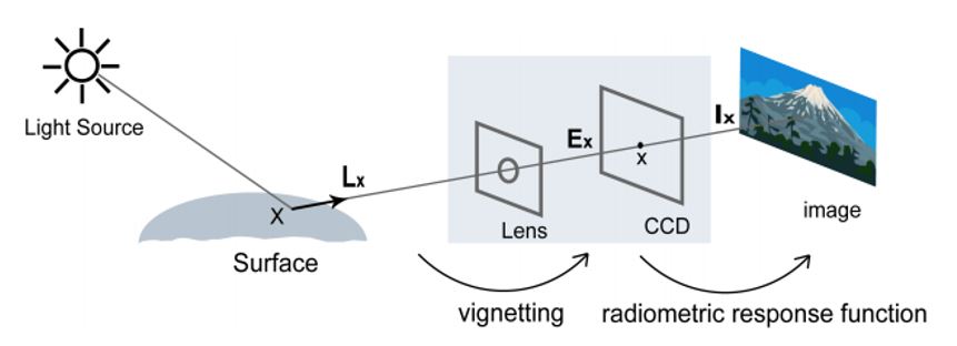
Figure 2a. The image formation process can be decomposed into two transformations: 1. Radiance from a scene to irradiance at the detector and 2. irradiance at the detector to image brightness in discretized signal counts. Falloff is often lumped into the blanket term, ‘vignetting’. Diagram of imaging pipeline by Seon Joo Kim.

Optical and Mechanical Vignetting

In optical vignetting, an off-axis ray bundle from an object is clipped by at the edge of one or more apertures within an imaging system. [3] While this condition is occasionally a design tradeoff to reduce aberrations or cost, optical vignetting diminishes the irradiance at the detector from off-axis object points. Optical vignetting can be avoided for many systems by design.

In mechanical vignetting, huge swaths of light are blocked by an external object such as a lens hood. The resulting image appears sharply truncated because radiant energy from the scene cannot reach portions of the entrance pupil. [4]. While remediating optical vignetting is possible, this is infeasible for mechanical vignetting due to extreme information loss.

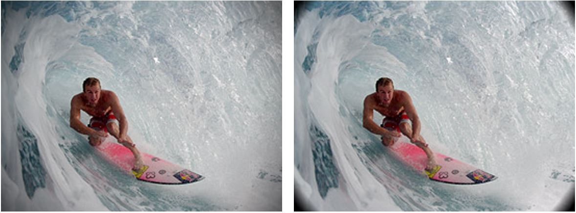
Figure 2b. In the image (left), the result of optical vignetting shows progressive falloff in pixel brightness level from center to corners. Mechanically vignetting the same image, this effect is far more abrupt since the corners of the sensor detect no light from the scene at all (right). 'Understanding Lens Vignetting' from RED, LLC.

Relative Illumination

Relative Illumination, or natural vignetting, describes the falloff of irradiance at a detector’s periphery due to radiometric effects. It is defined as the “ratio of irradiance in the focal plane at off-axis field positions to the irradiance at the center of the field”. [5]

While the illumination of the image plane is commonly associated with the famous \( cos^4 \theta\) law, where \(\theta\) is the oblique field angle measured from the optical axis, this is not generalizable towards all imaging systems. The well-known expression (shown below) only models how the irradiance at a small target area varies with \(\theta\), and distance z, from a small, distant Lambertian source. In the limit of a small aperture, the \( cos^4 \theta\) law can be extended to model the relative illumination of a pinhole camera, but is otherwise ungeneralizable.

$$ dE = L_{Lam, Uni} \frac{dA}{z^2}cos^4\theta$$

Reiss and Siew demonstrate that the differential irradiance \(dE\) also depends on a differential distortion factor, \(dD/dh\), or the instantaneous rate of change of image distortion with respect to object height. [6] [7] The irradiance on a small target area is specifically sensitive to non-constant areal magnification inherent to the imaging system. To illustrate the influence of differential distortion, Siew tunes the relative illumination profile for an otherwise static landscape lens design by changing the stop position alone.

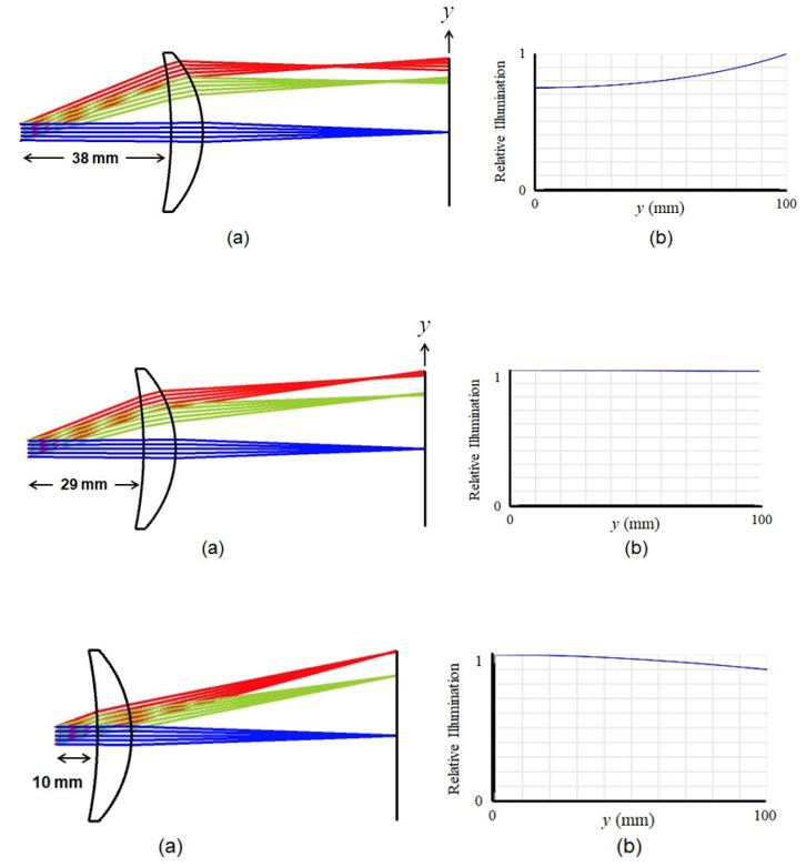
Figure 3. During the sweep of the position of a small aperture, all distortion remained as 1-5% barrel distortion, but the differential distortion flipped in sign. By changing the position of the stop, the relative illumination profile was tuned to near uniformity with ease. This example was given by Ronan Siew with extraordinary clarity and I highly recommend his book [8]

Finally, Reshidko and Sasián derive a general expression, to the fourth order, for what lens designers have known all along – separate aberrations can collectively combine to influence the relative illumination. Assuming a lossless system, the authors synthesize the irradiation transport equation and pupil aberration function to find a polynomial whose coefficients impact the relative illumination at the image focal plane. [9]

$$ Ri(\overrightarrow{H})+Ri_{200}(\overrightarrow{H} \cdot \overrightarrow{H}) +Ri_{400}(\overrightarrow{H} \cdot \overrightarrow{H})^2$$

The dependence on aberrations lies in two coefficients, \(Ri_{200}\) and \(Ri_{400}\), which each vary with sums of \( \bar{u'}^2\) and \( \bar{u'}^4\) weighted by Seidel coefficients, \( \bar{W}_{nlm}\), including that of coma, astigmatism, and distortion. The larger statement is that aberrations can alter the exit pupil dimensions to compensate for the relatively smaller flux contributions of oblique rays into the entrance pupil. Modifying the aberrations carefully, a more balanced illumination across the detector can be achieved with a systematic ray tracing methodology.

Origins and Models

The discussion up to now has sought to depict how illumination at a detector may vary so much from design intention or plausibly, manufacturing defects. In practicality, two image-processing based approaches (rather than ray tracing-based ones) are used in common practice. Both methods aggregate and compensate all falloff effects into a single correction operation for a raw image. “Flat Fielding” methods image a highly-controlled reference scene to generate a look-up table for pixel-wise correction. Vignetting Function Fitting uses a large series of images (i.e. adjacent, related through motion) to generate a ‘vignetting function’, which alters pixel brightness based a parametric dependence on distance from image center. [10]

Flat Field Correction

Scientific imaging communities, such as those in microscopy and astrometry, prefer flat field correction (FFC), since the fidelity of the adjusted images is more limited by resource availability than weaknesses inherent to the method.

In flat-fielding, a scene of constant radiance and uniform illumination is prepared and its image from the camera of interest is used to calculate a Look-up Table (LUT). [11] [12] If the reference scene is highly uniform and Lambertian and also uniformly illuminated, then all aberrant pixel response (including physical detector defects like dead pixels) and radial falloff towards edges should represent the undesired effects of the imaging system alone. Thus, the LUT is a captured picture whose manipulation provides a linear correction mapping. The rectification operations is as follows, [13]

\( I_{ref}\), is captured of a scene corresponding to the anticipated pixel brightness value, \(I_{ideal}\). At each pixel coordinate, a multiplicative correction factor is calculated, \(I_{LUT} (m,n)=I_{ideal}/I_{ref} (m,n) \). Taken all together, a LUT corrects for any raw captured image, \(I(m,n)\), with the linear operation, \(I'(m,n)=I_{LUT} (m,n) \cdot I(m,n) \).

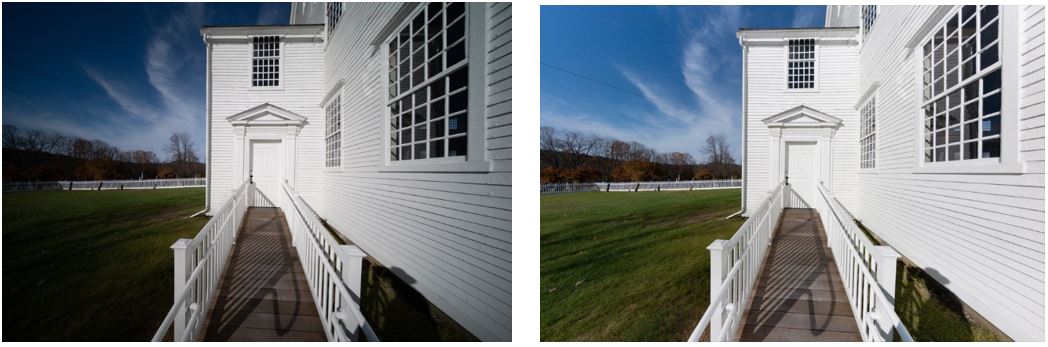
Figure 4. Sean Reid provides another example of before (left) and after FFC (right). Note that this linear transformation is only possible if the raw photographs were saved in linear steps. Data stored with gamma encoding cannot be directly linearly transformed with a LUT. [1]

In professional photography, some image quality image testing services recommend using of a large LCD monitor to generate uniform illumination and a slab of flashed opal glass to diffuse it. At the lower end, some hobbyists use paper mounted on boards, and at the higher end, engineered large lightbox diffusers with adjustable illuminance and uniformity (>95%) are available for purchase. [14] [15] Packages such as Adobe Lightroom, Imatest Master, and Raw Therapee enable flat-fielding correction.

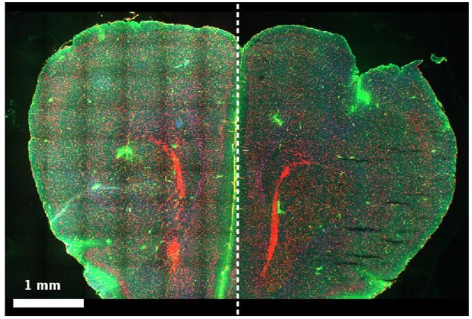
Figure 5. In microscopy, a homogenous fluorescence dye is to create the reference object for imaging. Here, this mosaic of microscopy image tiles shows stitching before (left) and after (right) flat field correction is applied using Huygens Stitching and Deconvolution software. [16]

In astrometry, low-signal fields are highly common and FFC methods must specifically consider dark signal non-uniformity. For imaging over a long exposure time, even cooled detectors will have pixels that show uncharacteristically high dark current. To prevent misinformation from this bias, a “dark count” image (viewing a dark and cold lens cap) must be taken over a long exposure and then time-averaged. This dark count is then subtracted from the raw image before applying the look-up table for FFC. [17]

Vignetting Function Fitting

The second rectification technique exists in a problem space such supposes that a flat-field calibration process is inaccessible. Exacerbating the lack of constraints even more, the exposure and camera response (i.e. linearity between detector irradiance and output signal) are sometimes unknown. Converting irradiance to pixel brightness level is modeled with the radiometric response function, \(f\). [2][10][18]

$$ I = f(k \cdot E) = f(k \cdot V(r) \cdot L)$$

$$ g = f^{-1}$$

Here, \(I\) is the pixel brightness, \(E\) is the irradiance at the detector, \(k\) is a constant related to exposure time, \(V(r)\) is the vignetting loss function as a function of distance from detector center, and L is the radiance of a science point in the direction of the camera. The objective is to find \(f\), \(g\), \(V(r)\), and \(k\) using a series of images of the same scene. The full treatment is far outside the scope of this paper, but estimating \(V(r)\) is briefly summarized. Since we can match feature points between images, we can identify pairs of points distant from the camera and approximate that they have the same radiance, or use information about pairs of points who share identical radii from the image center. With this information, we can roughly solve for f, the radiometric response function, and if we enforce a guess of the general fit for \(V(r)\), we can roughly decouple the vignetting function and then fit our information to obtain it.

From a survey of the modern literature, many common guesses for the vignetting function form assume a monotonic pixel brightness falloff towards the image edges. [2][18][19] Some variations of this method include hyperbolic cosines, but the most prominent form is an even polynomial series.

$$ V(r)= 1 + \sum_{n=1}^N c_n r^{2n}$$

If \(V(r)\), is known, then brightness count of each pixel within a captured image can be divided by it to undo this vignetting. While this guess is hardly given a physical basis in any of these papers, the popular vignetting loss function form is very similar (due to even polynomial dependence on radial distance from the center) to the relative illumination function suggested by Reshidko and Sasián.

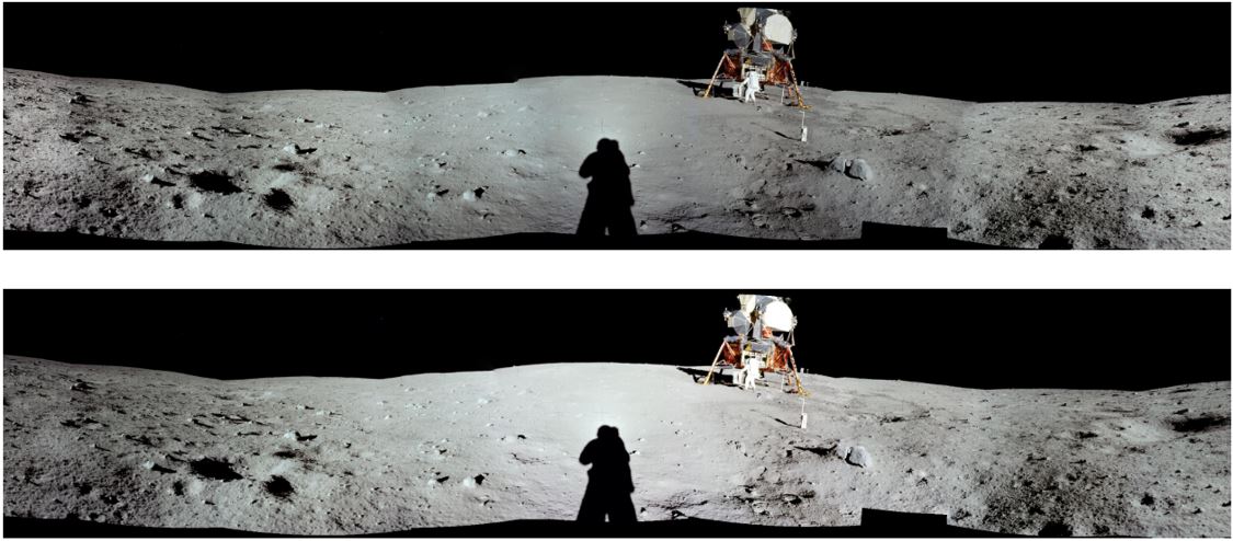
Figure 6. The benefits of using vignetting loss function before (above) and after (below) are best demonstrated in a real scenario where FFC would have been impractical to set up. By fitting a vignetting loss function to existing sequence of Apollo 11 photographs , Goldman removes vignetting artifacts previously present in a stitched panorama of the moon’s surface. [18]

While this correction method cannot account the full complexity of uneven illumination as the flat field method does, it is a beneficial model when many exposition parameters are unknown. Besides, this correction can easily be applied towards non-scientific photography to achieve effective illumination uniformity at low cost. For example, vignetting can be easily compensated in Adobe Photoshop and Lightroom without the need for a flat-field setup. In the case of commercial lenses, a user may use pre-existing lens profiles (an XML file containing lens correction parameters) made by the community or lens manufacturer to adjust their raw images. Adobe products officially use Goldman’s model, or the even polynomial expansion up to the 3rd order, for which, three scalar values are stored in the XML and tell a program how to correct each pixel, \(I(x_d,y_d )\), in the raw image for uneven illumination. [20]

$$ V(x_d,y_d) = 1 + \alpha_1 r_d^2 + \alpha_2 r_d^4 + \alpha_3 r_d^6 $$

$$ I'(x_d,y_d) = I(x_d,y_d)/V(x_d,y_d) $$

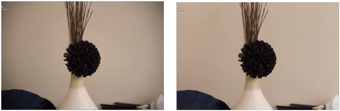
Figure 7. With the click of a single button, we can immediately reap the benefits of a using a vignetting model fitted to three coefficients. Corrections from an excellent Lightroom tutorial made by John Bodally. [18]

Conclusions

When a uniform scene is imaged, the irradiance falloff at the periphery of an image is due to a number of physical factors that imply uneven irradiance at the detector. This is popularly attributed to the popular cos4θ law, but non-uniform illumination can be the deliberate outcome of lens design and then significantly altered by aberrations from assembly errors. Ultimately, this combined effect ultimately detracts from an image’s suitability for panoramic stitching, validity in measurement, and aesthetic appeal. In practicality, we use two illumination uniformity rectification techniques: flat field calibration and vignetting loss function fitting. Both hold separate benefits and inconveniences depending on how well-compensated final image must be and what resources are available; however, both have been relatively successful in reducing undesired falloff for their end user analysis, synthesis, and perception. As requirements scale, it will be interesting if see how these methods will evolve into multidisciplinary solutions, such as including ray trace data for more customized lens profiles.

References

[1] S. Reid, “Adobe Flat Field for Lightroom Classic.” [Online]. Available: https://www.reidreviews.com/examples/flatfieldnew.html.
[2] S. J. Kim, “Radiometric Calibration Methods from Image Sequences,” University of North Carolina, Chapel Hill, 2008.
[3] J. E. Greivenkamp, Field Guide to Geometrical Optics. SPIE—The International Society for Optical Engineering, 2009.
[4] P. van Walree, “Vignetting,” 2009. [Online]. Available: http://www.cs.cmu.edu/~sensing-sensors/readings/vignetting.pdf.
[5] J. Sasián, “Radiometry in a Lens System,” Introd. to Lens Des., vol. 2, pp. 54–63, 2019.
[6] M. Reiss, “Notes on the Cos4 Law of Illumination,” J. Opt. Soc. Am., vol. 38, no. 11, pp. 980–986, 1948.
[7] R. Siew, “Relative illumination and image distortion,” Opt. Eng., vol. 56, no. 4, p. 049701, 2017.
[8] R. Siew, “Breaking Down The ‘ Cosine Fourth Power Law ,’” Vancouver, CA, 2019.
[9] D. Reshidko and J. Sasian, “The role of aberrations in the relative illumination of a lens system,” Nov. Opt. Syst. Des. Optim. XIX, vol. 9948, no. September 2016, p. 994806, 2016.
[10] P. Angelo, “Radiometric alignment and vignetting calibration,” Computer (Long. Beach. Calif)., pp. 1063–1082, 2007.
[11] P. Dinev, “LUTs : Take Control of Your Imaging Application,” 2006. [Online]. Available: https://www.techbriefs.com/component/content/article/tb/features/articles/12117?start=1.
[12] A. J. Norton, W. A. (W. A. Cooper, and Open University., Observing the universe : a guide to observational astronomy and planetary science. Open University, 2004.
[13] W. Yu, “Practical anti-vignetting methods for digital cameras,” IEEE Trans. Consum. Electron., vol. 50, no. 4, pp. 975–983, 2004.
[14] Imatest LLC, “Using Uniformity Part 1 | imatest,” Imatest Software Documentation v5.2, 2019. [Online]. Available: http://www.imatest.com/docs/uniformity/.
[15] A. Illumination, “DL071 Diffuse Light Specifications.” pp. 1–4, 2017.
[16] Scientific Volume Imaging B.V., “Huygens Professional User Guide for version 15.05,” 2015.
[17] M. R. Baril, “Flat field and dark frame correction,” The Pyxis CCD Camera Project, 2007. [Online]. Available: http://www.cfht.hawaii.edu/~baril/Pyxis/Help/flatdarkfield.html.
[18] D. B. Goldman, “Vignette and exposure calibration and compensation,” IEEE Trans. Pattern Anal. Mach. Intell., vol. 32, no. 12, pp. 2276–2288, 2010.
[19] W. Yu, “Practical anti-vignetting methods for digital cameras,” IEEE Trans. Consum. Electron., vol. 50, no. 4, pp. 975–983, Nov. 2004.
[20] S. Chen, H. Jin, J. Chien, E. Chan, and D. Goldman, “Adobe Camera Model,” 2010.